9.3 Perfect Competition in the Long Run
Learning Objectives
- Distinguish between economic profit and accounting profit.
- Explain why in long-run equilibrium in a perfectly competitive industry firms will earn zero economic profit.
- Describe the three possible effects on the costs of the factors of production that expansion or contraction of a perfectly competitive industry may have and illustrate the resulting long-run industry supply curve in each case.
- Explain why under perfection competition output prices will change by less than the change in production cost in the short run, but by the full amount of the change in production cost in the long run.
- Explain the effect of a change in fixed cost on price and output in the short run and in the long run under perfect competition.
In the long run, a firm is free to adjust all of its inputs. New firms can enter any market; existing firms can leave their markets. We shall see in this section that the model of perfect competition predicts that, at a long-run equilibrium, production takes place at the lowest possible cost per unit and that all economic profits and losses are eliminated.
Economic Profit and Economic Loss
Economic profits and losses play a crucial role in the model of perfect competition. The existence of economic profits in a particular industry attracts new firms to the industry in the long run. As new firms enter, the supply curve shifts to the right, price falls, and profits fall. Firms continue to enter the industry until economic profits fall to zero. If firms in an industry are experiencing economic losses, some will leave. The supply curve shifts to the left, increasing price and reducing losses. Firms continue to leave until the remaining firms are no longer suffering losses—until economic profits are zero.
Before examining the mechanism through which entry and exit eliminate economic profits and losses, we shall examine an important key to understanding it: the difference between the accounting and economic concepts of profit and loss.
Economic Versus Accounting Concepts of Profit and Loss
Economic profit equals total revenue minus total cost, where cost is measured in the economic sense as opportunity cost. An economic loss (negative economic profit) is incurred if total cost exceeds total revenue.
Accountants include only explicit costs in their computation of total cost. Explicit costs include charges that must be paid for factors of production such as labor and capital, together with an estimate of depreciation. Profit computed using only explicit costs is called accounting profit. It is the measure of profit firms typically report; firms pay taxes on their accounting profits, and a corporation reporting its profit for a particular period reports its accounting profits. To compute his accounting profits, Mr. Gortari, the radish farmer, would subtract explicit costs, such as charges for labor, equipment, and other supplies, from the revenue he receives.
Economists recognize costs in addition to the explicit costs listed by accountants. If Mr. Gortari were not growing radishes, he could be doing something else with the land and with his own efforts. Suppose the most valuable alternative use of his land would be to produce carrots, from which Mr. Gortari could earn $250 per month in accounting profits. The income he forgoes by not producing carrots is an opportunity cost of producing radishes. This cost is not explicit; the return Mr. Gortari could get from producing carrots will not appear on a conventional accounting statement of his accounting profit. A cost that is included in the economic concept of opportunity cost, but that is not an explicit cost, is called an implicit cost.
The Long Run and Zero Economic Profits
Given our definition of economic profits, we can easily see why, in perfect competition, they must always equal zero in the long run. Suppose there are two industries in the economy, and that firms in Industry A are earning economic profits. By definition, firms in Industry A are earning a return greater than the return available in Industry B. That means that firms in Industry B are earning less than they could in Industry A. Firms in Industry B are experiencing economic losses.
Given easy entry and exit, some firms in Industry B will leave it and enter Industry A to earn the greater profits available there. As they do so, the supply curve in Industry B will shift to the left, increasing prices and profits there. As former Industry B firms enter Industry A, the supply curve in Industry A will shift to the right, lowering profits in A. The process of firms leaving Industry B and entering A will continue until firms in both industries are earning zero economic profit. That suggests an important long-run result: Economic profits in a system of perfectly competitive markets will, in the long run, be driven to zero in all industries.
Eliminating Economic Profit: The Role of Entry
The process through which entry will eliminate economic profits in the long run is illustrated in Figure 9.14 “Eliminating Economic Profits in the Long Run”, which is based on the situation presented in Figure 9.7 “Applying the Marginal Decision Rule”. The price of radishes is $0.40 per pound. Mr. Gortari’s average total cost at an output of 6,700 pounds of radishes per month is $0.26 per pound. Profit per unit is $0.14 ($0.40 − $0.26). Mr. Gortari thus earns a profit of $938 per month (=$0.14 × 6,700).
Figure 9.14 Eliminating Economic Profits in the Long Run
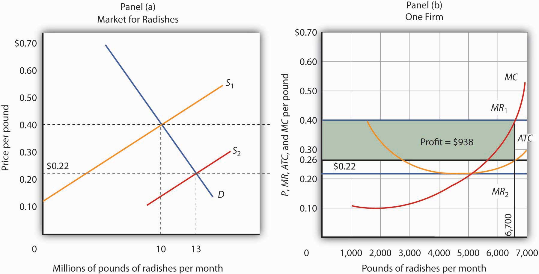
If firms in an industry are making an economic profit, entry will occur in the long run. In Panel (b), a single firm’s profit is shown by the shaded area. Entry continues until firms in the industry are operating at the lowest point on their respective average total cost curves, and economic profits fall to zero.
Profits in the radish industry attract entry in the long run. Panel (a) of Figure 9.14 “Eliminating Economic Profits in the Long Run” shows that as firms enter, the supply curve shifts to the right and the price of radishes falls. New firms enter as long as there are economic profits to be made—as long as price exceeds ATC in Panel (b). As price falls, marginal revenue falls to MR2 and the firm reduces the quantity it supplies, moving along the marginal cost (MC) curve to the lowest point on the ATC curve, at $0.22 per pound and an output of 5,000 pounds per month. Although the output of individual firms falls in response to falling prices, there are now more firms, so industry output rises to 13 million pounds per month in Panel (a).
Eliminating Losses: The Role of Exit
Just as entry eliminates economic profits in the long run, exit eliminates economic losses. In Figure 9.15 “Eliminating Economic Losses in the Long Run”, Panel (a) shows the case of an industry in which the market price P1 is below ATC. In Panel (b), at price P1 a single firm produces a quantity q1, assuming it is at least covering its average variable cost. The firm’s losses are shown by the shaded rectangle bounded by its average total cost C1 and price P1 and by output q1.
Because firms in the industry are losing money, some will exit. The supply curve in Panel (a) shifts to the left, and it continues shifting as long as firms are suffering losses. Eventually the supply curve shifts all the way to S2, price rises to P2, and economic profits return to zero.
Figure 9.15 Eliminating Economic Losses in the Long Run
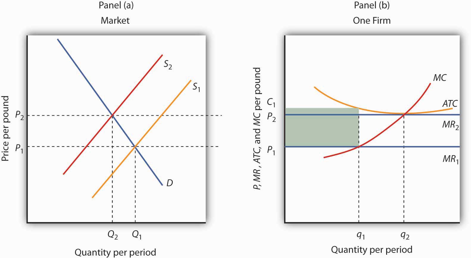
Panel (b) shows that at the initial price P1, firms in the industry cannot cover average total cost (MR1 is below ATC). That induces some firms to leave the industry, shifting the supply curve in Panel (a) to S2, reducing industry output to Q2 and raising price to P2. At that price (MR2), firms earn zero economic profit, and exit from the industry ceases. Panel (b) shows that the firm increases output from q1 to q2; total output in the market falls in Panel (a) because there are fewer firms. Notice that in Panel (a) quantity is designated by uppercase Q, while in Panel (b) quantity is designated by lowercase q. This convention is used throughout the text to distinguish between the quantity supplied in the market (Q) and the quantity supplied by a typical firm (q).
Entry, Exit, and Production Costs
In our examination of entry and exit in response to economic profit or loss in a perfectly competitive industry, we assumed that the ATC curve of a single firm does not shift as new firms enter or existing firms leave the industry. That is the case when expansion or contraction does not affect prices for the factors of production used by firms in the industry. When expansion of the industry does not affect the prices of factors of production, it is a constant-cost industry. In some cases, however, the entry of new firms may affect input prices.
As new firms enter, they add to the demand for the factors of production used by the industry. If the industry is a significant user of those factors, the increase in demand could push up the market price of factors of production for all firms in the industry. If that occurs, then entry into an industry will boost average costs at the same time as it puts downward pressure on price. Long-run equilibrium will still occur at a zero level of economic profit and with firms operating on the lowest point on the ATC curve, but that cost curve will be somewhat higher than before entry occurred. Suppose, for example, that an increase in demand for new houses drives prices higher and induces entry. That will increase the demand for workers in the construction industry and is likely to result in higher wages in the industry, driving up costs.
An industry in which the entry of new firms bids up the prices of factors of production and thus increases production costs is called an increasing-cost industry. As such an industry expands in the long run, its price will rise.
Some industries may experience reductions in input prices as they expand with the entry of new firms. That may occur because firms supplying the industry experience economies of scale as they increase production, thus driving input prices down. Expansion may also induce technological changes that lower input costs. That is clearly the case of the computer industry, which has enjoyed falling input costs as it has expanded. An industry in which production costs fall as firms enter in the long run is a decreasing-cost industry.
Just as industries may expand with the entry of new firms, they may contract with the exit of existing firms. In a constant-cost industry, exit will not affect the input prices of remaining firms. In an increasing-cost industry, exit will reduce the input prices of remaining firms. And, in a decreasing-cost industry, input prices may rise with the exit of existing firms.
The behavior of production costs as firms in an industry expand or reduce their output has important implications for the long-run industry supply curve, a curve that relates the price of a good or service to the quantity produced after all long-run adjustments to a price change have been completed. Every point on a long-run supply curve therefore shows a price and quantity supplied at which firms in the industry are earning zero economic profit. Unlike the short-run market supply curve, the long-run industry supply curve does not hold factor costs and the number of firms unchanged.
Figure 9.16 “Long-Run Supply Curves in Perfect Competition” shows three long-run industry supply curves. In Panel (a), SCC is a long-run supply curve for a constant-cost industry. It is horizontal. Neither expansion nor contraction by itself affects market price. In Panel (b), SIC is a long-run supply curve for an increasing-cost industry. It rises as the industry expands. In Panel (c), SDC is a long-run supply curve for a decreasing-cost industry. Its downward slope suggests a falling price as the industry expands.
Figure 9.16 Long-Run Supply Curves in Perfect Competition
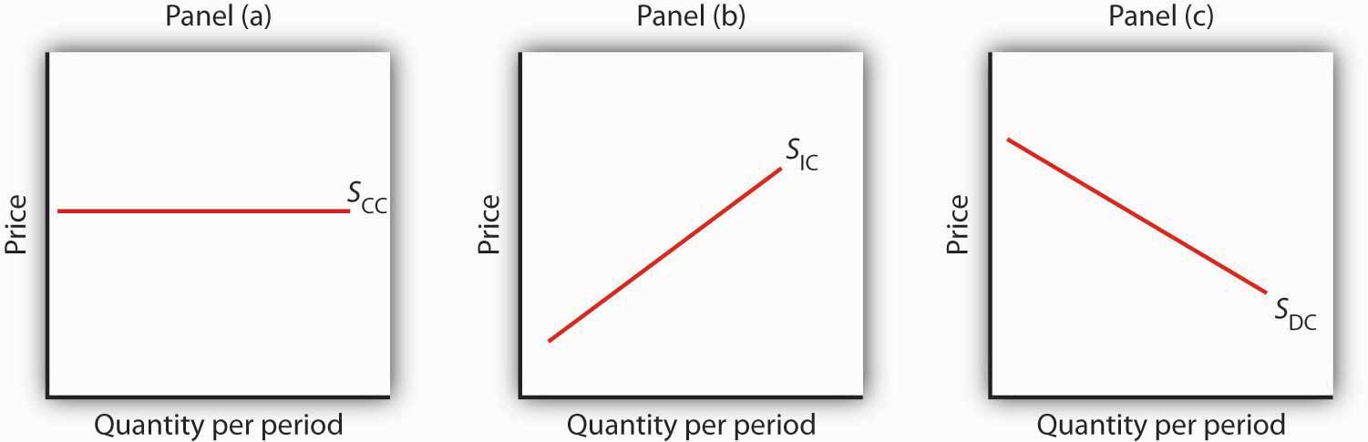
The long-run supply curve for a constant-cost, perfectly competitive industry is a horizontal line, SCC, shown in Panel (a). The long-run curve for an increasing-cost industry is an upward-sloping curve, SIC, as in Panel (b). The downward-sloping long-run supply curve, SDC, for a decreasing cost industry is given in Panel (c).
Changes in Demand and in Production Cost
The primary application of the model of perfect competition is in predicting how firms will respond to changes in demand and in production costs. To see how firms respond to a particular change, we determine how the change affects demand or cost conditions and then see how the profit-maximizing solution is affected in the short run and in the long run. Having determined how the profit-maximizing firms of the model would respond, we can then predict firms’ responses to similar changes in the real world.
In the examples that follow, we shall assume, for simplicity, that entry or exit do not affect the input prices facing firms in the industry. That is, we assume a constant-cost industry with a horizontal long-run industry supply curve similar to SCC in Figure 9.16 “Long-Run Supply Curves in Perfect Competition”. We shall assume that firms are covering their average variable costs, so we can ignore the possibility of shutting down.
Changes in Demand
Changes in demand can occur for a variety of reasons. There may be a change in preferences, incomes, the price of a related good, population, or consumer expectations. A change in demand causes a change in the market price, thus shifting the marginal revenue curves of firms in the industry.
Let us consider the impact of a change in demand for oats. Suppose new evidence suggests that eating oats not only helps to prevent heart disease, but also prevents baldness in males. This will, of course, increase the demand for oats. To assess the impact of this change, we assume that the industry is perfectly competitive and that it is initially in long-run equilibrium at a price of $1.70 per bushel. Economic profits equal zero.
The initial situation is depicted in Figure 9.17 “Short-Run and Long-Run Adjustments to an Increase in Demand”. Panel (a) shows that at a price of $1.70, industry output is Q1 (point A), while Panel (b) shows that the market price constitutes the marginal revenue, MR1, facing a single firm in the industry. The firm responds to that price by finding the output level at which the MC and MR1 curves intersect. That implies a level of output q1 at point A′.
The new medical evidence causes demand to increase to D2 in Panel (a). That increases the market price to $2.30 (point B), so the marginal revenue curve for a single firm rises to MR2 in Panel (b). The firm responds by increasing its output to q2 in the short run (point B′). Notice that the firm’s average total cost is slightly higher than its original level of $1.70; that is because of the U shape of the curve. The firm is making an economic profit shown by the shaded rectangle in Panel (b). Other firms in the industry will earn an economic profit as well, which, in the long run, will attract entry by new firms. New entry will shift the supply curve to the right; entry will continue as long as firms are making an economic profit. The supply curve in Panel (a) shifts to S2, driving the price down in the long run to the original level of $1.70 per bushel and returning economic profits to zero in long-run equilibrium. A single firm will return to its original level of output, q1 (point A′) in Panel (b), but because there are more firms in the industry, industry output rises to Q3 (point C) in Panel (a).
Figure 9.17 Short-Run and Long-Run Adjustments to an Increase in Demand
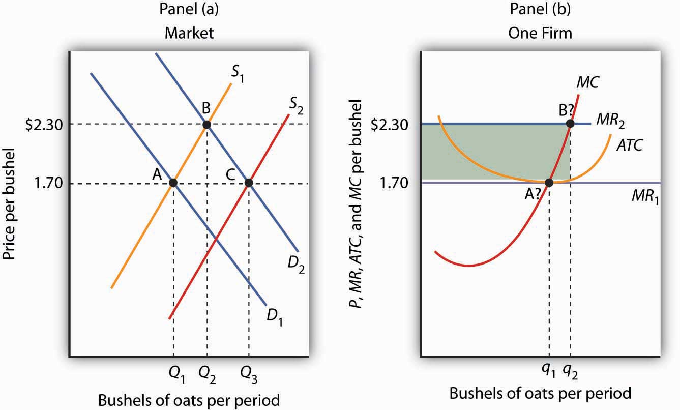
The initial equilibrium price and output are determined in the market for oats by the intersection of demand and supply at point A in Panel (a). An increase in the market demand for oats, from D1 to D2 in Panel (a), shifts the equilibrium solution to point B. The price increases in the short run from $1.70 per bushel to $2.30. Industry output rises to Q2. For a single firm, the increase in price raises marginal revenue from MR1 to MR2; the firm responds in the short run by increasing its output to q2. It earns an economic profit given by the shaded rectangle. In the long run, the opportunity for profit attracts new firms. In a constant-cost industry, the short-run supply curve shifts to S2; market equilibrium now moves to point C in Panel (a). The market price falls back to $1.70. The firm’s demand curve returns to MR1, and its output falls back to the original level, q1. Industry output has risen to Q3 because there are more firms.
A reduction in demand would lead to a reduction in price, shifting each firm’s marginal revenue curve downward. Firms would experience economic losses, thus causing exit in the long run and shifting the supply curve to the left. Eventually, the price would rise back to its original level, assuming changes in industry output did not lead to changes in input prices. There would be fewer firms in the industry, but each firm would end up producing the same output as before.
Changes in Production Cost
A firm’s costs change if the costs of its inputs change. They also change if the firm is able to take advantage of a change in technology. Changes in production cost shift the ATC curve. If a firm’s variable costs are affected, its marginal cost curves will shift as well. Any change in marginal cost produces a similar change in industry supply, since it is found by adding up marginal cost curves for individual firms.
Suppose a reduction in the price of oil reduces the cost of producing oil changes for automobiles. We shall assume that the oil-change industry is perfectly competitive and that it is initially in long-run equilibrium at a price of $27 per oil change, as shown in Panel (a) of Figure 9.18 “A Reduction in the Cost of Producing Oil Changes”. Suppose that the reduction in oil prices reduces the cost of an oil change by $3.
Figure 9.18 A Reduction in the Cost of Producing Oil Changes
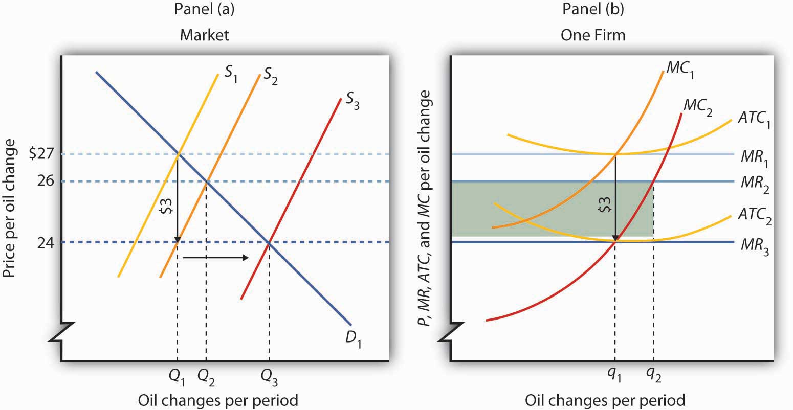
The initial equilibrium price, $27, and quantity, Q1, of automobile oil changes are determined by the intersection of market demand, D1, and market supply, S1 in Panel (a). The industry is in long-run equilibrium; a typical firm, shown in Panel (b), earns zero economic profit. A reduction in oil prices reduces the marginal and average total costs of producing an oil change by $3. The firm’s marginal cost curve shifts to MC2, and its average total cost curve shifts to ATC2. The short-run industry supply curve shifts down by $3 to S2. The market price falls to $26; the firm increases its output to q2 and earns an economic profit given by the shaded rectangle. In the long run, the opportunity for profit shifts the industry supply curve to S3. The price falls to $24, and the firm reduces its output to the original level, q1. It now earns zero economic profit once again. Industry output in Panel (a) rises to Q3 because there are more firms; price has fallen by the full amount of the reduction in production costs.
A reduction in production cost shifts the firm’s cost curves down. The firm’s average total cost and marginal cost curves shift down, as shown in Panel (b). In Panel (a) the supply curve shifts from S1 to S2. The industry supply curve is made up of the marginal cost curves of individual firms; because each of them has shifted downward by $3, the industry supply curve shifts downward by $3.
Notice that price in the short run falls to $26; it does not fall by the $3 reduction in cost. That is because the supply and demand curves are sloped. While the supply curve shifts downward by $3, its intersection with the demand curve falls by less than $3. The firm in Panel (b) responds to the lower price and lower cost by increasing output to q2, where MC2 and MR2 intersect. That leaves firms in the industry with an economic profit; the economic profit for the firm is shown by the shaded rectangle in Panel (b). Profits attract entry in the long run, shifting the supply curve to the right to S3 in Panel (a) Entry will continue as long as firms are making an economic profit—it will thus continue until the price falls by the full amount of the $3 reduction in cost. The price falls to $24, industry output rises to Q3, and the firm’s output returns to its original level, q1.
An increase in variable costs would shift the average total, average variable, and marginal cost curves upward. It would shift the industry supply curve upward by the same amount. The result in the short run would be an increase in price, but by less than the increase in cost per unit. Firms would experience economic losses, causing exit in the long run. Eventually, price would increase by the full amount of the increase in production cost.
Some cost increases will not affect marginal cost. Suppose, for example, that an annual license fee of $5,000 is imposed on firms in a particular industry. The fee is a fixed cost; it does not affect marginal cost. Imposing such a fee shifts the average total cost curve upward but causes no change in marginal cost. There is no change in price or output in the short run. Because firms are suffering economic losses, there will be exit in the long run. Prices ultimately rise by enough to cover the cost of the fee, leaving the remaining firms in the industry with zero economic profit.
Price will change to reflect whatever change we observe in production cost. A change in variable cost causes price to change in the short run. In the long run, any change in average total cost changes price by an equal amount.
The message of long-run equilibrium in a competitive market is a profound one. The ultimate beneficiaries of the innovative efforts of firms are consumers. Firms in a perfectly competitive world earn zero profit in the long-run. While firms can earn accounting profits in the long-run, they cannot earn economic profits.
Key Takeaways
- The economic concept of profit differs from accounting profit. The accounting concept deals only with explicit costs, while the economic concept of profit incorporates explicit and implicit costs.
- The existence of economic profits attracts entry, economic losses lead to exit, and in long-run equilibrium, firms in a perfectly competitive industry will earn zero economic profit.
- The long-run supply curve in an industry in which expansion does not change input prices (a constant-cost industry) is a horizontal line. The long-run supply curve for an industry in which production costs increase as output rises (an increasing-cost industry) is upward sloping. The long-run supply curve for an industry in which production costs decrease as output rises (a decreasing-cost industry) is downward sloping.
- In a perfectly competitive market in long-run equilibrium, an increase in demand creates economic profit in the short run and induces entry in the long run; a reduction in demand creates economic losses (negative economic profits) in the short run and forces some firms to exit the industry in the long run.
- When production costs change, price will change by less than the change in production cost in the short run. Price will adjust to reflect fully the change in production cost in the long run.
- A change in fixed cost will have no effect on price or output in the short run. It will induce entry or exit in the long run so that price will change by enough to leave firms earning zero economic profit.
Try It!
Consider Acme Clothing’s situation in the second Try It! in this chapter. Suppose this situation is typical of firms in the jacket market. Explain what will happen in the market for jackets in the long run, assuming nothing happens to the prices of factors of production used by firms in the industry. What will happen to the equilibrium price? What is the equilibrium level of economic profits?
Case in Point: Competition in the Market for Generic Prescription Drugs

Generic prescription drugs are essentially identical substitutes for more expensive brand-name prescription drugs. Since the passage of the Drug Competition and Patent Term Restoration Act of 1984 (commonly referred to as the Hatch-Waxman Act) made it easier for manufacturers to enter the market for generic drugs, the generic drug industry has taken off. Generic drugs represented 19% of the prescription drug industry in 1984 and today represent more than half of the industry. U.S. generic sales were $15 billion in 2002 and soared to $192 billion in 2006. In 2006, the average price of a branded prescription was $111.02 compared to $32.23 for a generic prescription.
A Congressional Budget Office study in the late 1990s showed that entry into the generic drug industry has been the key to this price differential. As shown in the table, when there are one to five manufacturers selling generic copies of a given branded drug, the ratio of the generic price to the branded price is about 60%. With more than 20 competitors, the ratio falls to about 40%.
The generic drug industry is largely characterized by the attributes of a perfectly competitive market. Competitors have good information about the product and sell identical products. The largest generic drug manufacturer in the CBO study had a 16% share of the generic drug manufacturing industry, but most generic manufacturers’ sales constituted only 1% to 5% of the market. The 1984 legislation eased entry into this market. And, as the model of perfect competition predicts, entry has driven prices down, benefiting consumers to the tune of tens of billions of dollars each year.
Table 9.1 Price Comparison of Generic and Innovator Drugs, by Number of Manufacturers
| Number of Generic Manufacturers of a Given Innovator Drug | Number of Innovator Drugs in Category | Avg. Rx Price, All Generic Drugs in Category | Avg. Rx Price, All Innovator Drugs in Category | Avg. Ratio of the Generic Price to the Innovator Price for Same Drug |
|---|---|---|---|---|
| 1 to 5 | 34 | $23.40 | $37.20 | 0.61 |
| 6 to 10 | 26 | $26.40 | $42.60 | 0.61 |
| 11 to 15 | 29 | $20.90 | $50.20 | 0.42 |
| 16 to 20 | 19 | $19.90 | $45.00 | 0.46 |
| 21 to 24 | 4 | $11.50 | $33.90 | 0.39 |
| Average | $22.40 | $43.00 | 0.53 | |
Sources: Congressional Budget Office, “How Increased Competition from Generic Drugs Has Affected Prices and Returns in the Pharmaceutical Industry,” July 1998. Available at www.cbo.gov; “Generic Pharmaceutical Industry Anticipates Double-Digit Growth,” PR Newswire, March 17, 2004. Available at www.Prnewswire.com; 2008 Statistical Abstract of the United States, Table 130.
Answer to Try It! Problem
The availability of economic profits will attract new firms to the jacket industry in the long run, shifting the market supply curve to the right. Entry will continue until economic profits are eliminated. The price will fall; Acme’s marginal revenue curve shifts down. The equilibrium level of economic profits in the long run is zero.
