8.1 Production Choices and Costs: The Short Run
Learning Objectives
- Understand the terms associated with the short-run production function—total product, average product, and marginal product—and explain and illustrate how they are related to each other.
- Explain the concepts of increasing, diminishing, and negative marginal returns and explain the law of diminishing marginal returns.
- Understand the terms associated with costs in the short run—total variable cost, total fixed cost, total cost, average variable cost, average fixed cost, average total cost, and marginal cost—and explain and illustrate how they are related to each other.
- Explain and illustrate how the product and cost curves are related to each other and to determine in what ranges on these curves marginal returns are increasing, diminishing, or negative.
Our analysis of production and cost begins with a period economists call the short run. The short run in this microeconomic context is a planning period over which the managers of a firm must consider one or more of their factors of production as fixed in quantity. For example, a restaurant may regard its building as a fixed factor over a period of at least the next year. It would take at least that much time to find a new building or to expand or reduce the size of its present facility. Decisions concerning the operation of the restaurant during the next year must assume the building will remain unchanged. Other factors of production could be changed during the year, but the size of the building must be regarded as a constant.
When the quantity of a factor of production cannot be changed during a particular period, it is called a fixed factor of production. For the restaurant, its building is a fixed factor of production for at least a year. A factor of production whose quantity can be changed during a particular period is called a variable factor of production; factors such as labor and food are examples.
While the managers of the restaurant are making choices concerning its operation over the next year, they are also planning for longer periods. Over those periods, managers may contemplate alternatives such as modifying the building, building a new facility, or selling the building and leaving the restaurant business. The planning period over which a firm can consider all factors of production as variable is called the long run.
At any one time, a firm will be making both short-run and long-run choices. The managers may be planning what to do for the next few weeks and for the next few years. Their decisions over the next few weeks are likely to be short-run choices. Decisions that will affect operations over the next few years may be long-run choices, in which managers can consider changing every aspect of their operations. Our analysis in this section focuses on the short run. We examine long-run choices later in this chapter.
The Short-Run Production Function
A firm uses factors of production to produce a product. The relationship between factors of production and the output of a firm is called a production function Our first task is to explore the nature of the production function.
Consider a hypothetical firm, Acme Clothing, a shop that produces jackets. Suppose that Acme has a lease on its building and equipment. During the period of the lease, Acme’s capital is its fixed factor of production. Acme’s variable factors of production include things such as labor, cloth, and electricity. In the analysis that follows, we shall simplify by assuming that labor is Acme’s only variable factor of production.
Total, Marginal, and Average Products
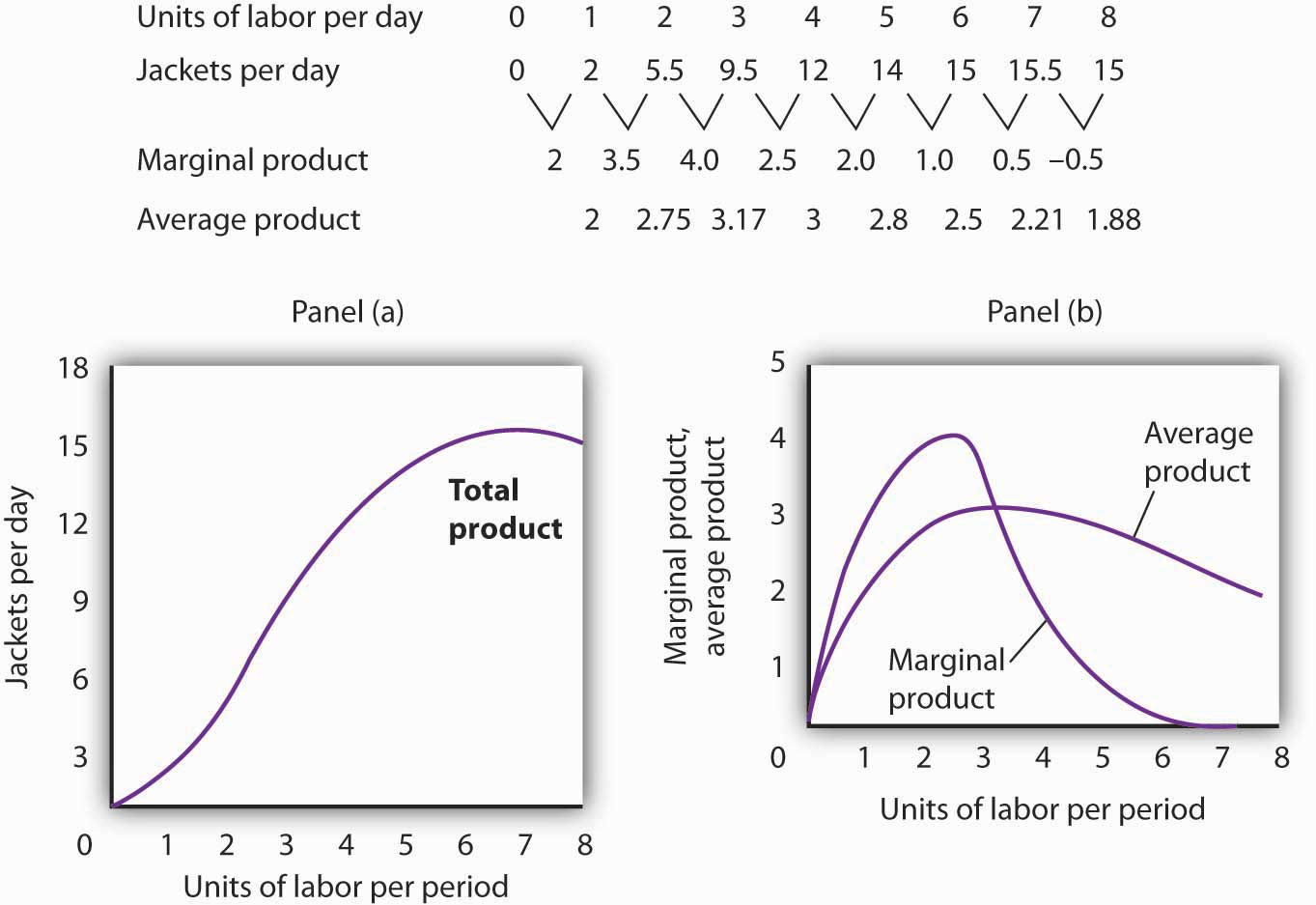
Figure 8.1 “Acme Clothing’s Total Product Curve” shows the number of jackets Acme can obtain with varying amounts of labor (in this case, tailors) and its given level of capital. A total product curve shows the quantities of output that can be obtained from different amounts of a variable factor of production, assuming other factors of production are fixed.
Figure 8.1 Acme Clothing’s Total Product Curve
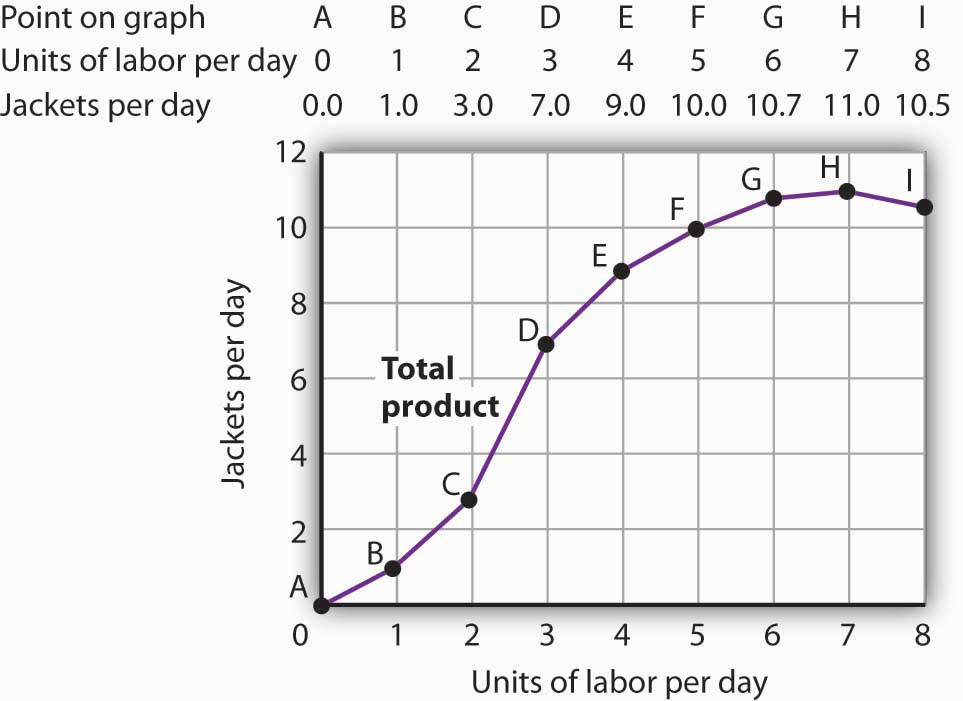
The table gives output levels per day for Acme Clothing Company at various quantities of labor per day, assuming the firm’s capital is fixed. These values are then plotted graphically as a total product curve.
Notice what happens to the slope of the total product curve in Figure 8.1 “Acme Clothing’s Total Product Curve”. Between 0 and 3 units of labor per day, the curve becomes steeper. Between 3 and 7 workers, the curve continues to slope upward, but its slope diminishes. Beyond the seventh tailor, production begins to decline and the curve slopes downward.
We measure the slope of any curve as the vertical change between two points divided by the horizontal change between the same two points. The slope of the total product curve for labor equals the change in output (ΔQ) divided by the change in units of labor (ΔL):
Slope of the total product curve = ΔQ/ΔL
The slope of a total product curve for any variable factor is a measure of the change in output associated with a change in the amount of the variable factor, with the quantities of all other factors held constant. The amount by which output rises with an additional unit of a variable factor is the marginal product of the variable factor. Mathematically, marginal product is the ratio of the change in output to the change in the amount of a variable factor. The marginal product of labor (MPL), for example, is the amount by which output rises with an additional unit of labor. It is thus the ratio of the change in output to the change in the quantity of labor (ΔQ/ΔL), all other things unchanged. It is measured as the slope of the total product curve for labor.
Equation 8.1
[latex]MP_L = \Delta Q/ \Delta L[/latex]
In addition we can define the average product of a variable factor. It is the output per unit of variable factor. The average product of labor (APL), for example, is the ratio of output to the number of units of labor (Q/L).
Equation 8.2
[latex]AP_L = Q/L[/latex]
The concept of average product is often used for comparing productivity levels over time or in comparing productivity levels among nations. When you read in the newspaper that productivity is rising or falling, or that productivity in the United States is nine times greater than productivity in China, the report is probably referring to some measure of the average product of labor.
The total product curve in Panel (a) of Figure 8.2 “From Total Product to the Average and Marginal Product of Labor” is repeated from Figure 8.1 “Acme Clothing’s Total Product Curve”. Panel (b) shows the marginal product and average product curves. Notice that marginal product is the slope of the total product curve, and that marginal product rises as the slope of the total product curve increases, falls as the slope of the total product curve declines, reaches zero when the total product curve achieves its maximum value, and becomes negative as the total product curve slopes downward. As in other parts of this text, marginal values are plotted at the midpoint of each interval. The marginal product of the fifth unit of labor, for example, is plotted between 4 and 5 units of labor. Also notice that the marginal product curve intersects the average product curve at the maximum point on the average product curve. When marginal product is above average product, average product is rising. When marginal product is below average product, average product is falling.
Figure 8.2 From Total Product to the Average and Marginal Product of Labor
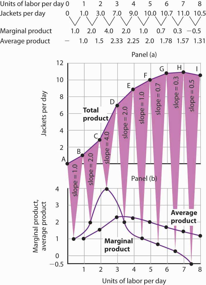
The first two rows of the table give the values for quantities of labor and total product from Figure 8.1 “Acme Clothing’s Total Product Curve”. Marginal product, given in the third row, is the change in output resulting from a one-unit increase in labor. Average product, given in the fourth row, is output per unit of labor. Panel (a) shows the total product curve. The slope of the total product curve is marginal product, which is plotted in Panel (b). Values for marginal product are plotted at the midpoints of the intervals. Average product rises and falls. Where marginal product is above average product, average product rises. Where marginal product is below average product, average product falls. The marginal product curve intersects the average product curve at the maximum point on the average product curve.
As a student you can use your own experience to understand the relationship between marginal and average values. Your grade point average (GPA) represents the average grade you have earned in all your course work so far. When you take an additional course, your grade in that course represents the marginal grade. What happens to your GPA when you get a grade that is higher than your previous average? It rises. What happens to your GPA when you get a grade that is lower than your previous average? It falls. If your GPA is a 3.0 and you earn one more B, your marginal grade equals your GPA and your GPA remains unchanged.
The relationship between average product and marginal product is similar. However, unlike your course grades, which may go up and down willy-nilly, marginal product always rises and then falls, for reasons we will explore shortly. As soon as marginal product falls below average product, the average product curve slopes downward. While marginal product is above average product, whether marginal product is increasing or decreasing, the average product curve slopes upward.
As we have learned, maximizing behavior requires focusing on making decisions at the margin. For this reason, we turn our attention now toward increasing our understanding of marginal product.
Increasing, Diminishing, and Negative Marginal Returns
Adding the first worker increases Acme’s output from 0 to 1 jacket per day. The second tailor adds 2 jackets to total output; the third adds 4. The marginal product goes up because when there are more workers, each one can specialize to a degree. One worker might cut the cloth, another might sew the seams, and another might sew the buttonholes. Their increasing marginal products are reflected by the increasing slope of the total product curve over the first 3 units of labor and by the upward slope of the marginal product curve over the same range. The range over which marginal products are increasing is called the range of increasing marginal returns. Increasing marginal returns exist in the context of a total product curve for labor, so we are holding the quantities of other factors constant. Increasing marginal returns may occur for any variable factor.
The fourth worker adds less to total output than the third; the marginal product of the fourth worker is 2 jackets. The data in Figure 8.2 “From Total Product to the Average and Marginal Product of Labor” show that marginal product continues to decline after the fourth worker as more and more workers are hired. The additional workers allow even greater opportunities for specialization, but because they are operating with a fixed amount of capital, each new worker adds less to total output. The fifth tailor adds only a single jacket to total output. When each additional unit of a variable factor adds less to total output, the firm is experiencing diminishing marginal returns. Over the range of diminishing marginal returns, the marginal product of the variable factor is positive but falling. Once again, we assume that the quantities of all other factors of production are fixed. Diminishing marginal returns may occur for any variable factor. Panel (b) shows that Acme experiences diminishing marginal returns between the third and seventh workers, or between 7 and 11 jackets per day.
After the seventh unit of labor, Acme’s fixed plant becomes so crowded that adding another worker actually reduces output. When additional units of a variable factor reduce total output, given constant quantities of all other factors, the company experiences negative marginal returns. Now the total product curve is downward sloping, and the marginal product curve falls below zero. Figure 8.3 “Increasing Marginal Returns, Diminishing Marginal Returns, and Negative Marginal Returns” shows the ranges of increasing, diminishing, and negative marginal returns. Clearly, a firm will never intentionally add so much of a variable factor of production that it enters a range of negative marginal returns.
Figure 8.3 Increasing Marginal Returns, Diminishing Marginal Returns, and Negative Marginal Returns
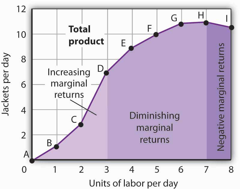
This graph shows Acme’s total product curve from Figure 8.1 “Acme Clothing’s Total Product Curve” with the ranges of increasing marginal returns, diminishing marginal returns, and negative marginal returns marked. Acme experiences increasing marginal returns between 0 and 3 units of labor per day, diminishing marginal returns between 3 and 7 units of labor per day, and negative marginal returns beyond the 7th unit of labor.
The idea that the marginal product of a variable factor declines over some range is important enough, and general enough, that economists state it as a law. The law of diminishing marginal returns holds that the marginal product of any variable factor of production will eventually decline, assuming the quantities of other factors of production are unchanged.
Heads Up!
It is easy to confuse the concept of diminishing marginal returns with the idea of negative marginal returns. To say a firm is experiencing diminishing marginal returns is not to say its output is falling. Diminishing marginal returns mean that the marginal product of a variable factor is declining. Output is still increasing as the variable factor is increased, but it is increasing by smaller and smaller amounts. As we saw in Figure 8.2 “From Total Product to the Average and Marginal Product of Labor” and Figure 8.3 “Increasing Marginal Returns, Diminishing Marginal Returns, and Negative Marginal Returns”, the range of diminishing marginal returns was between the third and seventh workers; over this range of workers, output rose from 7 to 11 jackets. Negative marginal returns started after the seventh worker.
To see the logic of the law of diminishing marginal returns, imagine a case in which it does not hold. Say that you have a small plot of land for a vegetable garden, 10 feet by 10 feet in size. The plot itself is a fixed factor in the production of vegetables. Suppose you are able to hold constant all other factors—water, sunshine, temperature, fertilizer, and seed—and vary the amount of labor devoted to the garden. How much food could the garden produce? Suppose the marginal product of labor kept increasing or was constant. Then you could grow an unlimited quantity of food on your small plot—enough to feed the entire world! You could add an unlimited number of workers to your plot and still increase output at a constant or increasing rate. If you did not get enough output with, say, 500 workers, you could use 5 million; the five-millionth worker would add at least as much to total output as the first. If diminishing marginal returns to labor did not occur, the total product curve would slope upward at a constant or increasing rate.
The shape of the total product curve and the shape of the resulting marginal product curve drawn in Figure 8.2 “From Total Product to the Average and Marginal Product of Labor” are typical of any firm for the short run. Given its fixed factors of production, increasing the use of a variable factor will generate increasing marginal returns at first; the total product curve for the variable factor becomes steeper and the marginal product rises. The opportunity to gain from increased specialization in the use of the variable factor accounts for this range of increasing marginal returns. Eventually, though, diminishing returns will set in. The total product curve will become flatter, and the marginal product curve will fall.
Costs in the Short Run
A firm’s costs of production depend on the quantities and prices of its factors of production. Because we expect a firm’s output to vary with the firm’s use of labor in a specific way, we can also expect the firm’s costs to vary with its output in a specific way. We shall put our information about Acme’s product curves to work to discover how a firm’s costs vary with its level of output.
We distinguish between the costs associated with the use of variable factors of production, which are called variable costs, and the costs associated with the use of fixed factors of production, which are called fixed costs. For most firms, variable costs includes costs for raw materials, salaries of production workers, and utilities. The salaries of top management may be fixed costs; any charges set by contract over a period of time, such as Acme’s one-year lease on its building and equipment, are likely to be fixed costs. A term commonly used for fixed costs is overhead. Notice that fixed costs exist only in the short run. In the long run, the quantities of all factors of production are variable, so that all long-run costs are variable.
Total variable cost (TVC) is cost that varies with the level of output. Total fixed cost (TFC) is cost that does not vary with output. Total cost (TC) is the sum of total variable cost and total fixed cost:
Equation 8.3
[latex]TVC + TFC = TC[/latex]
From Total Production to Total Cost
Next we illustrate the relationship between Acme’s total product curve and its total costs. Acme can vary the quantity of labor it uses each day, so the cost of this labor is a variable cost. We assume capital is a fixed factor of production in the short run, so its cost is a fixed cost.
Suppose that Acme pays a wage of $100 per worker per day. If labor is the only variable factor, Acme’s total variable costs per day amount to $100 times the number of workers it employs. We can use the information given by the total product curve, together with the wage, to compute Acme’s total variable costs.
We know from Figure 8.1 “Acme Clothing’s Total Product Curve” that Acme requires 1 worker working 1 day to produce 1 jacket. The total variable cost of a jacket thus equals $100. Three units of labor produce 7 jackets per day; the total variable cost of 7 jackets equals $300. Figure 8.4 “Computing Variable Costs” shows Acme’s total variable costs for producing each of the output levels given in Figure 8.1 “Acme Clothing’s Total Product Curve”
Figure 8.4 “Computing Variable Costs” gives us costs for several quantities of jackets, but we need a bit more detail. We know, for example, that 7 jackets have a total variable cost of $300. What is the total variable cost of 6 jackets?
Figure 8.4 Computing Variable Costs
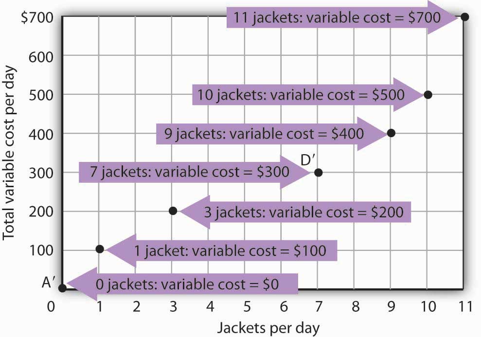
The points shown give the variable costs of producing the quantities of jackets given in the total product curve in Figure 8.1 “Acme Clothing’s Total Product Curve” and Figure 8.2 “From Total Product to the Average and Marginal Product of Labor”. Suppose Acme’s workers earn $100 per day. If Acme produces 0 jackets, it will use no labor—its variable cost thus equals $0 (Point A′). Producing 7 jackets requires 3 units of labor; Acme’s variable cost equals $300 (Point D′).
We can estimate total variable costs for other quantities of jackets by inspecting the total product curve in Figure 8.1 “Acme Clothing’s Total Product Curve”. Reading over from a quantity of 6 jackets to the total product curve and then down suggests that the Acme needs about 2.8 units of labor to produce 6 jackets per day. Acme needs 2 full-time and 1 part-time tailors to produce 6 jackets. Figure 8.5 “The Total Variable Cost Curve” gives the precise total variable costs for quantities of jackets ranging from 0 to 11 per day. The numbers in boldface type are taken from Figure 8.4 “Computing Variable Costs”; the other numbers are estimates we have assigned to produce a total variable cost curve that is consistent with our total product curve. You should, however, be certain that you understand how the numbers in boldface type were found.
Figure 8.5 The Total Variable Cost Curve
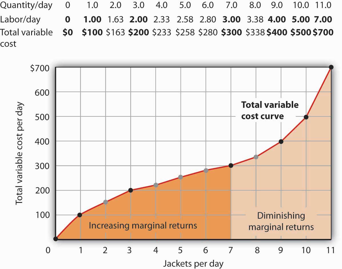
Total variable costs for output levels shown in Acme’s total product curve were shown in Figure 8.4 “Computing Variable Costs”. To complete the total variable cost curve, we need to know the variable cost for each level of output from 0 to 11 jackets per day. The variable costs and quantities of labor given in Figure 8.4 “Computing Variable Costs” are shown in boldface in the table here and with black dots in the graph. The remaining values were estimated from the total product curve in Figure 8.1 “Acme Clothing’s Total Product Curve” and Figure 8.2 “From Total Product to the Average and Marginal Product of Labor”. For example, producing 6 jackets requires 2.8 workers, for a variable cost of $280.
Suppose Acme’s present plant, including the building and equipment, is the equivalent of 20 units of capital. Acme has signed a long-term lease for these 20 units of capital at a cost of $200 per day. In the short run, Acme cannot increase or decrease its quantity of capital—it must pay the $200 per day no matter what it does. Even if the firm cuts production to zero, it must still pay $200 per day in the short run.
Acme’s total cost is its total fixed cost of $200 plus its total variable cost. We add $200 to the total variable cost curve in Figure 8.5 “The Total Variable Cost Curve” to get the total cost curve shown in Figure 8.6 “From Variable Cost to Total Cost”.
Figure 8.6 From Variable Cost to Total Cost
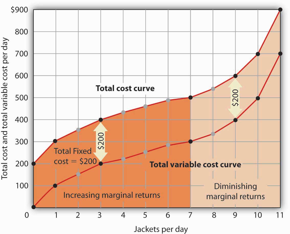
We add total fixed cost to the total variable cost to obtain total cost. In this case, Acme’s total fixed cost equals $200 per day.
Notice something important about the shapes of the total cost and total variable cost curves in Figure 8.6 “From Variable Cost to Total Cost”. The total cost curve, for example, starts at $200 when Acme produces 0 jackets—that is its total fixed cost. The curve rises, but at a decreasing rate, up to the seventh jacket. Beyond the seventh jacket, the curve becomes steeper and steeper. The slope of the total variable cost curve behaves in precisely the same way.
Recall that Acme experienced increasing marginal returns to labor for the first three units of labor—or the first seven jackets. Up to the third worker, each additional worker added more and more to Acme’s output. Over the range of increasing marginal returns, each additional jacket requires less and less additional labor. The first jacket required one tailor; the second required the addition of only a part-time tailor; the third required only that Acme boost that part-time tailor’s hours to a full day. Up to the seventh jacket, each additional jacket requires less and less additional labor, and thus costs rise at a decreasing rate; the total cost and total variable cost curves become flatter over the range of increasing marginal returns.
Acme experiences diminishing marginal returns beyond the third unit of labor—or the seventh jacket. Notice that the total cost and total variable cost curves become steeper and steeper beyond this level of output. In the range of diminishing marginal returns, each additional unit of a factor adds less and less to total output. That means each additional unit of output requires larger and larger increases in the variable factor, and larger and larger increases in costs.
Marginal and Average Costs
Marginal and average cost curves, which will play an important role in the analysis of the firm, can be derived from the total cost curve. Marginal cost shows the additional cost of each additional unit of output a firm produces. This is a specific application of the general concept of marginal cost presented earlier. Given the marginal decision rule’s focus on evaluating choices at the margin, the marginal cost curve takes on enormous importance in the analysis of a firm’s choices. The second curve we shall derive shows the firm’s average total cost at each level of output. Average total cost (ATC) is total cost divided by quantity; it is the firm’s total cost per unit of output:
Equation 8.4
[latex]ATC = TC/Q[/latex]
We shall also discuss average variable costs (AVC), which is the firm’s variable cost per unit of output; it is total variable cost divided by quantity:
Equation 8.5
[latex]AVC = TVC/Q[/latex]
We are still assessing the choices facing the firm in the short run, so we assume that at least one factor of production is fixed. Finally, we will discuss average fixed cost (AFC), which is total fixed cost divided by quantity:
Equation 8.6
[latex]AFC = TFC/Q[/latex]
Marginal cost (MC) is the amount by which total cost rises with an additional unit of output. It is the ratio of the change in total cost to the change in the quantity of output:
Equation 8.7
[latex]MC = \Delta TC/ \Delta Q[/latex]
It equals the slope of the total cost curve. Figure 8.7 “Total Cost and Marginal Cost” shows the same total cost curve that was presented in Figure 8.6 “From Variable Cost to Total Cost”. This time the slopes of the total cost curve are shown; these slopes equal the marginal cost of each additional unit of output. For example, increasing output from 6 to 7 units (ΔQ=1) increases total cost from $480 to $500 (ΔTC=$20). The seventh unit thus has a marginal cost of $20 (ΔTC/ΔQ=$20/1=$20). Marginal cost falls over the range of increasing marginal returns and rises over the range of diminishing marginal returns.
Heads Up!
Notice that the various cost curves are drawn with the quantity of output on the horizontal axis. The various product curves are drawn with quantity of a factor of production on the horizontal axis. The reason is that the two sets of curves measure different relationships. Product curves show the relationship between output and the quantity of a factor; they therefore have the factor quantity on the horizontal axis. Cost curves show how costs vary with output and thus have output on the horizontal axis.
Figure 8.7 Total Cost and Marginal Cost
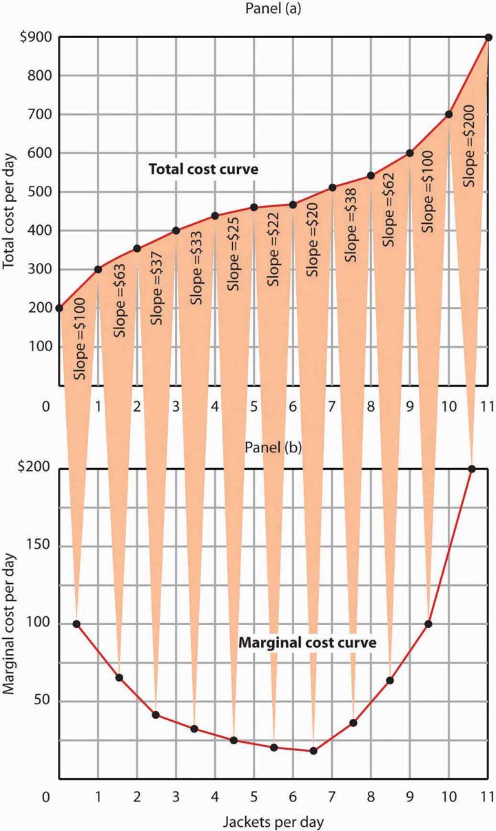
Marginal cost in Panel (b) is the slope of the total cost curve in Panel (a).
Figure 8.8 “Marginal Cost, Average Fixed Cost, Average Variable Cost, and Average Total Cost in the Short Run” shows the computation of Acme’s short-run average total cost, average variable cost, and average fixed cost and graphs of these values. Notice that the curves for short-run average total cost and average variable cost fall, then rise. We say that these cost curves are U-shaped. Average fixed cost keeps falling as output increases. This is because the fixed costs are spread out more and more as output expands; by definition, they do not vary as labor is added. Since average total cost (ATC) is the sum of average variable cost (AVC) and average fixed cost (AFC), i.e.,
Equation 8.8
[latex]AVC + AFC = ATC[/latex]
the distance between the ATC and AVC curves keeps getting smaller and smaller as the firm spreads its overhead costs over more and more output.
Figure 8.8 Marginal Cost, Average Fixed Cost, Average Variable Cost, and Average Total Cost in the Short Run
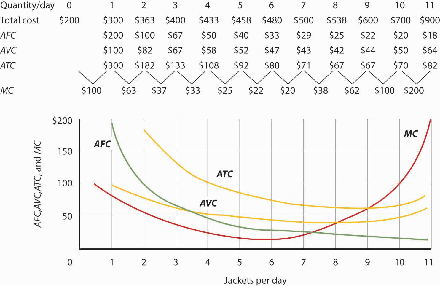
Total cost figures for Acme Clothing are taken from Figure 8.7 “Total Cost and Marginal Cost”. The other values are derived from these. Average total cost (ATC) equals total cost divided by quantity produced; it also equals the sum of the average fixed cost (AFC) and average variable cost (AVC) (exceptions in table are due to rounding to the nearest dollar); average variable cost is variable cost divided by quantity produced. The marginal cost (MC) curve (from Figure 8.7 “Total Cost and Marginal Cost”) intersects the ATC and AVC curves at the lowest points on both curves. The AFC curve falls as quantity increases.
Figure 8.8 “Marginal Cost, Average Fixed Cost, Average Variable Cost, and Average Total Cost in the Short Run” includes the marginal cost data and the marginal cost curve from Figure 8.7 “Total Cost and Marginal Cost”. The marginal cost curve intersects the average total cost and average variable cost curves at their lowest points. When marginal cost is below average total cost or average variable cost, the average total and average variable cost curves slope downward. When marginal cost is greater than short-run average total cost or average variable cost, these average cost curves slope upward. The logic behind the relationship between marginal cost and average total and variable costs is the same as it is for the relationship between marginal product and average product.
We turn next in this chapter to an examination of production and cost in the long run, a planning period in which the firm can consider changing the quantities of any or all factors.
Key Takeaways
Figure 8.9
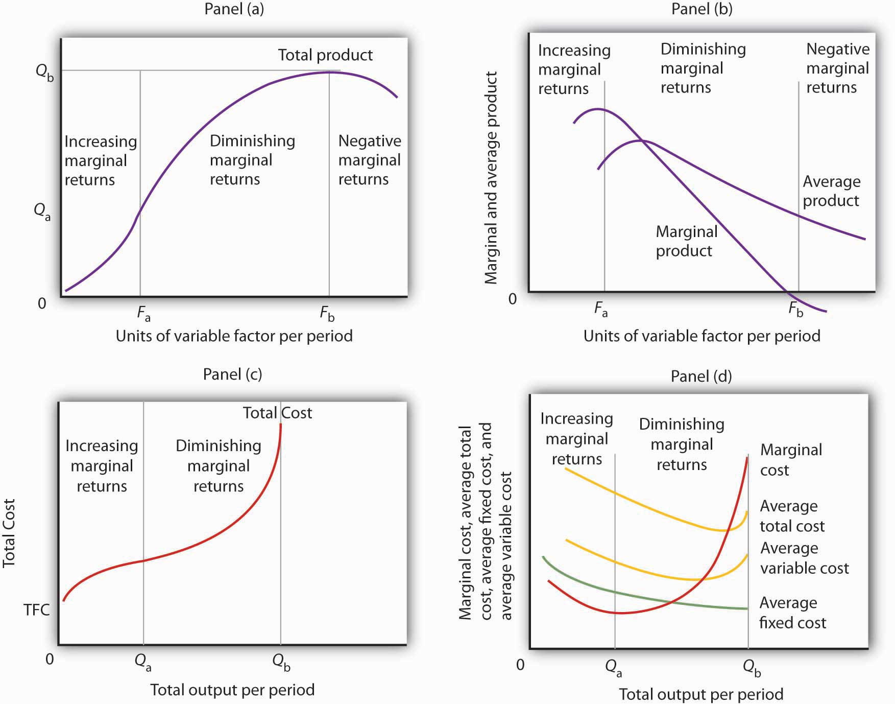
- In Panel (a), the total product curve for a variable factor in the short run shows that the firm experiences increasing marginal returns from zero to Fa units of the variable factor (zero to Qa units of output), diminishing marginal returns from Fa to Fb (Qa to Qb units of output), and negative marginal returns beyond Fb units of the variable factor.
- Panel (b) shows that marginal product rises over the range of increasing marginal returns, falls over the range of diminishing marginal returns, and becomes negative over the range of negative marginal returns. Average product rises when marginal product is above it and falls when marginal product is below it.
- In Panel (c), total cost rises at a decreasing rate over the range of output from zero to Qa This was the range of output that was shown in Panel (a) to exhibit increasing marginal returns. Beyond Qa, the range of diminishing marginal returns, total cost rises at an increasing rate. The total cost at zero units of output (shown as the intercept on the vertical axis) is total fixed cost.
- Panel (d) shows that marginal cost falls over the range of increasing marginal returns, then rises over the range of diminishing marginal returns. The marginal cost curve intersects the average total cost and average variable cost curves at their lowest points. Average fixed cost falls as output increases. Note that average total cost equals average variable cost plus average fixed cost.
-
Assuming labor is the variable factor of production, the following definitions and relations describe production and cost in the short run:
[latex]MP_L = \Delta Q/ \Delta L[/latex]
[latex]AP_L = Q/L[/latex]
[latex]TVC + TFC = TC[/latex]
[latex]ATC = TC/Q[/latex]
[latex]AVC = TVC/Q[/latex]
[latex]AFC = TFC/Q[/latex]
[latex]MC = \Delta TC/ \Delta Q[/latex]
Try It!
-
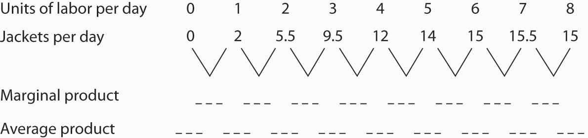
Suppose Acme gets some new equipment for producing jackets. The table below gives its new production function. Compute marginal product and average product and fill in the bottom two rows of the table. Referring to Figure 8.2 “From Total Product to the Average and Marginal Product of Labor”, draw a graph showing Acme’s new total product curve. On a second graph, below the one showing the total product curve you drew, sketch the marginal and average product curves. Remember to plot marginal product at the midpoint between each input level. On both graphs, shade the regions where Acme experiences increasing marginal returns, diminishing marginal returns, and negative marginal returns.
Figure 8.10
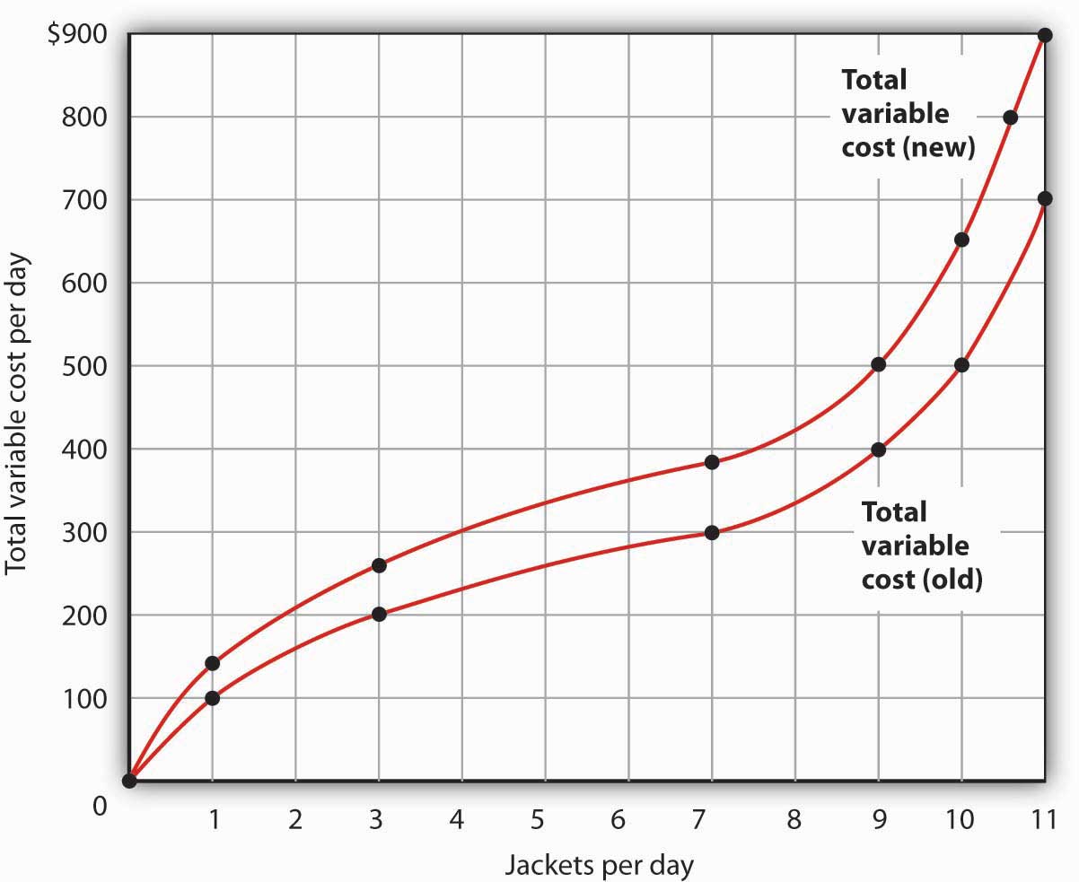
- Draw the points showing total variable cost at daily outputs of 0, 1, 3, 7, 9, 10, and 11 jackets per day when Acme faced a wage of $100 per day. (Use Figure 8.5 “The Total Variable Cost Curve” as a model.) Sketch the total variable cost curve as shown in Figure 8.4 “Computing Variable Costs”. Now suppose that the wage rises to $125 per day. On the same graph, show the new points and sketch the new total variable cost curve. Explain what has happened. What will happen to Acme’s marginal cost curve? Its average total, average variable, and average fixed cost curves? Explain.

Case in Point: The Production of Fitness
Figure 8.11
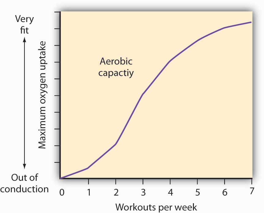
How much should an athlete train?
Sports physiologists often measure the “total product” of training as the increase in an athlete’s aerobic capacity—the capacity to absorb oxygen into the bloodstream. An athlete can be thought of as producing aerobic capacity using a fixed factor (his or her natural capacity) and a variable input (exercise). The chart shows how this aerobic capacity varies with the number of workouts per week. The curve has a shape very much like a total product curve—which, after all, is precisely what it is.
The data suggest that an athlete experiences increasing marginal returns from exercise for the first three days of training each week; indeed, over half the total gain in aerobic capacity possible is achieved. A person can become even more fit by exercising more, but the gains become smaller with each added day of training. The law of diminishing marginal returns applies to training.
The increase in fitness that results from the sixth and seventh workouts each week is small. Studies also show that the costs of daily training, in terms of increased likelihood of injury, are high. Many trainers and coaches now recommend that athletes—at all levels of competition—take a day or two off each week.
Source: Jeff Galloway, Galloway’s Book on Running (Bolinas, CA: Shelter Publications, 2002), p. 56.
Answers to Try It! Problems
Figure 8.12
- The increased wage will shift the total variable cost curve upward; the old and new points and the corresponding curves are shown at the right.
- The total variable cost curve has shifted upward because the cost of labor, Acme’s variable factor, has increased. The marginal cost curve shows the additional cost of each additional unit of output a firm produces. Because an increase in output requires more labor, and because labor now costs more, the marginal cost curve will shift upward. The increase in total variable cost will increase total cost; average total and average variable costs will rise as well. Average fixed cost will not change.
Figure 8.13