21.1 Measuring Total Output
Learning Objectives
- Define gross domestic product and its four major spending components and illustrate the various flows using the circular flow model.
- Distinguish between measuring GDP as the sum of the values of final goods and services and as the sum of values added at each stage of production.
- Distinguish between gross domestic product and gross national product.
An economy produces a mind-boggling array of goods and services. In 2007, for example, Domino’s Pizza produced 400 million pizzas. The United States Steel Corporation, the nation’s largest steel company, produced 23.6 million tons of steel. Strong Brothers Lumber Co., a Colorado firm, produced 2.1 million board feet of lumber. The Louisiana State University football team drew 722,166 fans to its home games—and won the national championship. Leonor Montenegro, a pediatric nurse in Los Angeles, delivered 387 babies and took care of 233 additional patients. A list of all the goods and services produced in any year would be virtually endless.
So—what kind of year was 2007? We would not get very far trying to wade through a list of all the goods and services produced that year. It is helpful to have instead a single number that measures total output in the economy; that number is GDP.
The Components of GDP
We can divide the goods and services produced during any period into four broad components, based on who buys them. These components of GDP are personal consumption (C), gross private domestic investment (I), government purchases (G), and net exports (Xn). Thus
Equation 21.1
[latex]\small GDP = consumption \: (C) + private \: investment \: (I) + government \: purchases \: (G) + net \: exports \: (X_n)[/latex]
[latex]GDP = C + I + G + X_n[/latex]
We will examine each of these components, and we will see how each fits into the pattern of macroeconomic activity. Before we begin, it will be helpful to distinguish between two types of variables: stocks and flows. A flow variable is a variable that is measured over a specific period of time. A stock variable is a variable that is independent of time. Income is an example of a flow variable. To say one’s income is, for example, $1,000 is meaningless without a time dimension. Is it $1,000 per hour? Per day? Per week? Per month? Until we know the time period, we have no idea what the income figure means. The balance in a checking account is an example of a stock variable. When we learn that the balance in a checking account is $1,000, we know precisely what that means; we do not need a time dimension. We will see that stock and flow variables play very different roles in macroeconomic analysis.
Personal Consumption
Personal consumption is a flow variable that measures the value of goods and services purchased by households during a time period. Purchases by households of groceries, health-care services, clothing, and automobiles—all are counted as consumption.
The production of consumer goods and services accounts for about 70% of total output. Because consumption is such a large part of GDP, economists seeking to understand the determinants of GDP must pay special attention to the determinants of consumption. In a later chapter we will explore these determinants and the impact of consumption on economic activity.
Personal consumption represents a demand for goods and services placed on firms by households. In the chapter on demand and supply, we saw how this demand could be presented in a circular flow model of the economy. Figure 21.1 “Personal Consumption in the Circular Flow” presents a circular flow model for an economy that produces only personal consumption goods and services. (We will add the other components of GDP to the circular flow as we discuss them.) Spending for these goods flows from households to firms; it is the arrow labeled “Personal consumption.” Firms produce these goods and services using factors of production: labor, capital, and natural resources. These factors are ultimately owned by households. The production of goods and services thus generates income to households; we see this income as the flow from firms to households labeled “Factor incomes” in the exhibit.
Figure 21.1 Personal Consumption in the Circular Flow
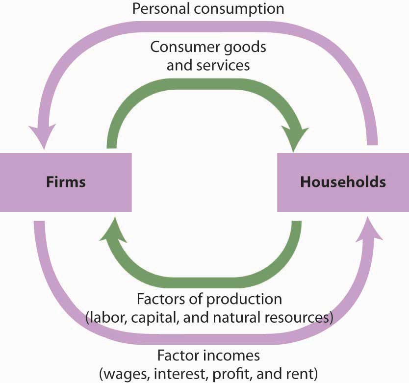
Personal consumption spending flows from households to firms. In return, consumer goods and services flow from firms to households. To produce the goods and services households demand, firms employ factors of production owned by households. There is thus a flow of factor services from households to firms, and a flow of payments of factor incomes from firms to households.
In exchange for payments that flow from households to firms, there is a flow of consumer goods and services from firms to households. This flow is shown in Figure 21.1 “Personal Consumption in the Circular Flow” as an arrow going from firms to households. When you buy a soda, for example, your payment to the store is part of the flow of personal consumption; the soda is part of the flow of consumer goods and services that goes from the store to a household—yours.
Similarly, the lower arrow in Figure 21.1 “Personal Consumption in the Circular Flow” shows the flow of factors of production—labor, capital, and natural resources—from households to firms. If you work for a firm, your labor is part of this flow. The wages you receive are part of the factor incomes that flow from firms to households.
There is a key difference in our interpretation of the circular flow picture in Figure 21.1 “Personal Consumption in the Circular Flow” from our analysis of the same model in the demand and supply chapter. There, our focus was microeconomics, which examines individual units of the economy. In thinking about the flow of consumption spending from households to firms, we emphasized demand and supply in particular markets—markets for such things as blue jeans, haircuts, and apartments. In thinking about the flow of income payments from firms to households, we focused on the demand and supply for particular factors of production, such as textile workers, barbers, and apartment buildings. Because our focus now is macroeconomics, the study of aggregates of economic activity, we will think in terms of the total of personal consumption and the total of payments to households.
Private Investment
Gross private domestic investment is the value of all goods produced during a period for use in the production of other goods and services. Like personal consumption, gross private domestic investment is a flow variable. It is often simply referred to as “private investment.” A hammer produced for a carpenter is private investment. A printing press produced for a magazine publisher is private investment, as is a conveyor-belt system produced for a manufacturing firm. Capital includes all the goods that have been produced for use in producing other goods; it is a stock variable. Private investment is a flow variable that adds to the stock of capital during a period.
Heads Up!
The term “investment” can generate confusion. In everyday conversation, we use the term “investment” to refer to uses of money to earn income. We say we have invested in a stock or invested in a bond. Economists, however, restrict “investment” to activities that increase the economy’s stock of capital. The purchase of a share of stock does not add to the capital stock; it is not investment in the economic meaning of the word. We refer to the exchange of financial assets, such as stocks or bonds, as financial investment to distinguish it from the creation of capital that occurs as the result of investment. Only when new capital is produced does investment occur. Confusing the economic concept of private investment with the concept of financial investment can cause misunderstanding of the way in which key components of the economy relate to one another.
Gross private domestic investment includes three flows that add to or maintain the nation’s capital stock: expenditures by business firms on new buildings, plants, tools, equipment, and software that will be used in the production of goods and services; expenditures on new residential housing; and changes in business inventories. Any addition to a firm’s inventories represents an addition to investment; a reduction subtracts from investment. For example, if a clothing store stocks 1,000 pairs of jeans, the jeans represent an addition to inventory and are part of gross private domestic investment. As the jeans are sold, they are subtracted from inventory and thus subtracted from investment.
By recording additions to inventories as investment and reductions from inventories as subtractions from investment, the accounting for GDP records production in the period in which it occurs. Suppose, for example, that Levi Strauss manufactures 1 million pairs of jeans late in 2007 and distributes them to stores at the end of December. The jeans will be added to inventory; they thus count as investment in 2007 and enter GDP for that year. Suppose they are sold in January 2008. They will be counted as consumption in GDP for 2008 but subtracted from inventory, and from investment. Thus, the production of the jeans will add to GDP in 2007, when they were produced. They will not count in 2008, save for any increase in the value of the jeans resulting from the services provided by the retail stores that sold them.
Private investment accounts for about 16% of GDP and at times even less. Despite its relatively small share of total economic activity, private investment plays a crucial role in the macroeconomy for two reasons:
- Private investment represents a choice to forgo current consumption in order to add to the capital stock of the economy. Private investment therefore adds to the economy’s capacity to produce and shifts its production possibilities curve outward. Investment is thus one determinant of economic growth, which is explored in another chapter.
- Private investment is a relatively volatile component of GDP; it can change dramatically from one year to the next. Fluctuations in GDP are often driven by fluctuations in private investment. We will examine the determinants of private investment in a chapter devoted to the study of investment.
Private investment represents a demand placed on firms for the production of capital goods. While it is a demand placed on firms, it flows from firms. In the circular flow model in Figure 21.2 “Private Investment in the Circular Flow”, we see a flow of investment going from firms to firms. The production of goods and services for consumption generates factor incomes to households; the production of capital goods for investment generates income to households as well.
Figure 21.2 Private Investment in the Circular Flow
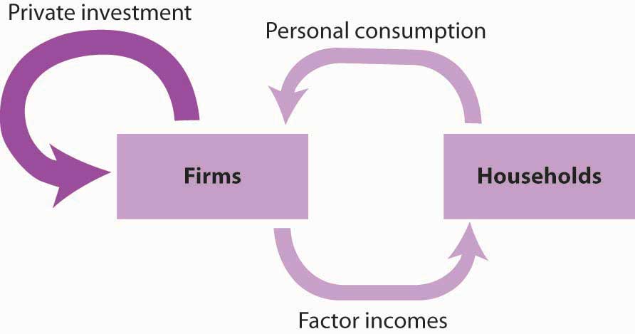
Private investment constitutes a demand placed on firms by other firms. It also generates factor incomes for households. To simplify the diagram, only the spending flows are shown—the corresponding flows of goods and services have been omitted.
Figure 21.2 “Private Investment in the Circular Flow” shows only spending flows and omits the physical flows represented by the arrows in Figure 21.1 “Personal Consumption in the Circular Flow”. This simplification will make our analysis of the circular flow model easier. It will also focus our attention on spending flows, which are the flows we will be studying.
Government Purchases
Government agencies at all levels purchase goods and services from firms. They purchase office equipment, vehicles, buildings, janitorial services, and so on. Many government agencies also produce goods and services. Police departments produce police protection. Public schools produce education. The National Aeronautics and Space Administration (NASA) produces space exploration.
Government purchases are the sum of purchases of goods and services from firms by government agencies plus the total value of output produced by government agencies themselves during a time period. Government purchases make up about 20% of GDP.
Government purchases are not the same thing as government spending. Much government spending takes the form of transfer payments, which are payments that do not require the recipient to produce a good or service in order to receive them. Transfer payments include Social Security and other types of assistance to retired people, welfare payments to poor people, and unemployment compensation to people who have lost their jobs. Transfer payments are certainly significant—they account for roughly half of all federal government spending in the United States. They do not count in a nation’s GDP, because they do not reflect the production of a good or service.
Government purchases represent a demand placed on firms, represented by the flow shown in Figure 21.3 “Government Purchases in the Circular Flow”. Like all the components of GDP, the production of goods and services for government agencies creates factor incomes for households.
Figure 21.3 Government Purchases in the Circular Flow
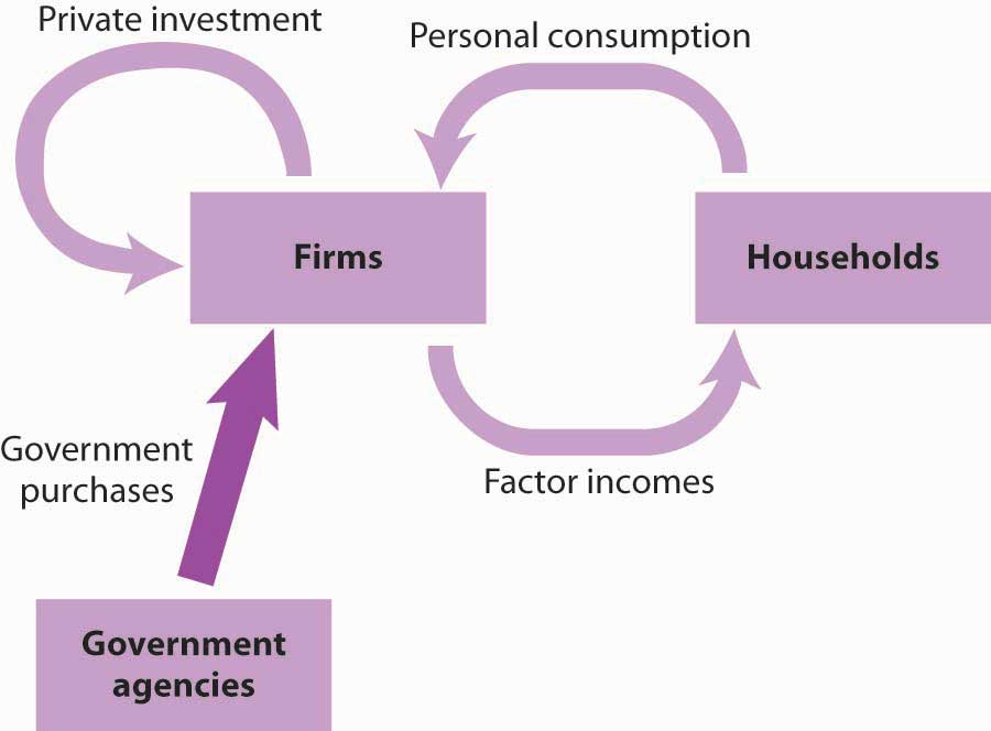
Purchases of goods and services by government agencies create demands on firms. As firms produce these goods and services, they create factor incomes for households.
Net Exports
Sales of a country’s goods and services to buyers in the rest of the world during a particular time period represent its exports. A purchase by a Japanese buyer of a Ford Taurus produced in the United States is a U.S. export. Exports also include such transactions as the purchase of accounting services from a New York accounting firm by a shipping line based in Hong Kong or the purchase of a ticket to Disney World by a tourist from Argentina. Imports are purchases of foreign-produced goods and services by a country’s residents during a period. United States imports include such transactions as the purchase by Americans of cars produced in Japan or tomatoes grown in Mexico or a stay in a French hotel by a tourist from the United States. Subtracting imports from exports yields net exports.
Equation 21.2
[latex]Exports \: (X) - imports \: (M) = net \: exports \: (X_n)[/latex]
In the third quarter of 2010, foreign buyers purchased $1,847.0 billion worth of goods and services from the United States. In the same year, U.S. residents, firms, and government agencies purchased $2,339.1 billion worth of goods and services from foreign countries. The difference between these two figures, −$552.2 billion, represented the net exports of the U.S. economy in the third quarter of 2010. Net exports were negative because imports exceeded exports. Negative net exports constitute a trade deficit. The amount of the deficit is the amount by which imports exceed exports. When exports exceed imports there is a trade surplus. The magnitude of the surplus is the amount by which exports exceed imports.
The United States has recorded more deficits than surpluses since World War II, but the amounts have typically been relatively small, only a few billion dollars. The trade deficit began to soar, however, in the 1980s and again in the 2000s. We will examine the reasons for persistent trade deficits in another chapter. The rest of the world plays a key role in the domestic economy and, as we will see later in the book, there is nothing particularly good or bad about trade surpluses or deficits. Goods and services produced for export represent roughly 13% of GDP, and the goods and services the United States imports add significantly to our standard of living.
In the circular flow diagram in Figure 21.4 “Net Exports in the Circular Flow”, net exports are shown with an arrow connecting firms to the rest of the world. The balance between the flows of exports and imports is net exports. When there is a trade surplus, net exports are positive and add spending to the circular flow. A trade deficit implies negative net exports; spending flows from firms to the rest of the world.
Figure 21.4 Net Exports in the Circular Flow
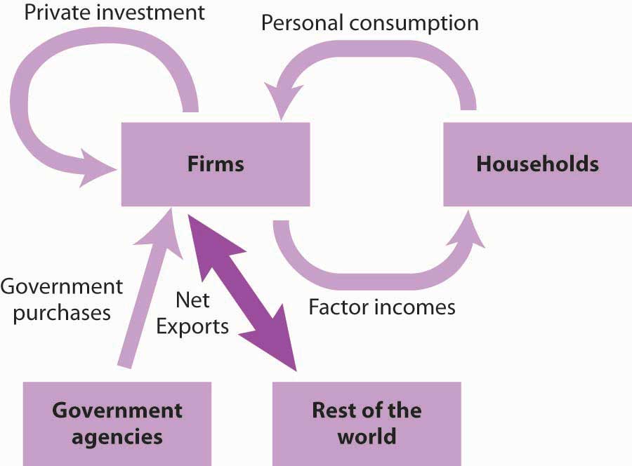
Net exports represent the balance between exports and imports. Net exports can be positive or negative. If they are positive, net export spending flows from the rest of the world to firms. If they are negative, spending flows from firms to the rest of the world.
The production of goods and services for personal consumption, private investment, government purchases, and net exports makes up a nation’s GDP. Firms produce these goods and services in response to demands from households (personal consumption), from other firms (private investment), from government agencies (government purchases), and from the rest of the world (net exports). All of this production creates factor income for households. Figure 21.5 “Spending in the Circular Flow Model” shows the circular flow model for all the spending flows we have discussed. Each flow is numbered for use in the exercise at the end of this section.
Figure 21.5 Spending in the Circular Flow Model
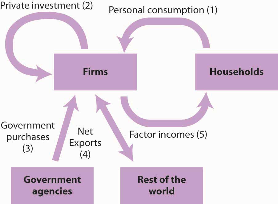
GDP equals the sum of production by firms of goods and services for personal consumption (1), private investment (2), government purchases (3), and net exports (4). The circular flow model shows these flows and shows that the production of goods and services generates factor incomes (5) to households.
The circular flow model identifies some of the forces at work in the economy, forces that we will be studying in later chapters. For example, an increase in any of the flows that place demands on firms (personal consumption, private investment, government purchases, and exports) will induce firms to expand their production. This effect is characteristic of the expansion phase of the business cycle. An increase in production will require firms to employ more factors of production, which will create more income for households. Households are likely to respond with more consumption, which will induce still more production, more income, and still more consumption. Similarly, a reduction in any of the demands placed on firms will lead to a reduction in output, a reduction in firms’ use of factors of production, a reduction in household incomes, a reduction in income, and so on. This sequence of events is characteristic of the contraction phase of the business cycle. Much of our work in macroeconomics will involve an analysis of the forces that prompt such changes in demand and an examination of the economy’s response to them.
Figure 21.6 “Components of GDP, 2010 (Q3) in Billions of Dollars” shows the size of the components of GDP in 2010. We see that the production of goods and services for personal consumption accounted for about 70% of GDP. Imports exceeded exports, so net exports were negative.
Figure 21.6 Components of GDP, 2010 (Q3) in Billions of Dollars
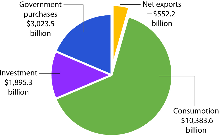
Consumption makes up the largest share of GDP. Net exports were negative in 2010. Total GDP—the sum of personal consumption, private investment, government purchases, and net exports—equaled $14,750.2 billion in 2010.
Source:
Bureau of Economic Analysis, National Income and Product Accounts, Table 1.1.5 (December 2010)
Final Goods and Value Added
GDP is the total value of all final goods and services produced during a particular period valued at prices in that period. That is not the same as the total value of all goods and services produced during a period. This distinction gives us another method of estimating GDP in terms of output.
Suppose, for example, that a logger cuts some trees and sells the logs to a sawmill. The mill makes lumber and sells it to a construction firm, which builds a house. The market price for the lumber includes the value of the logs; the price of the house includes the value of the lumber. If we try to estimate GDP by adding the value of the logs, the lumber, and the house, we would be counting the lumber twice and the logs three times. This problem is called “double counting,” and the economists who compute GDP seek to avoid it.
In the case of logs used for lumber and lumber produced for a house, GDP would include the value of the house. The lumber and the logs would not be counted as additional production because they are intermediate goods that were produced for use in building the house.
Another approach to estimating the value of final production is to estimate for each stage of production the value added, the amount by which the value of a firm’s output exceeds the value of the goods and services the firm purchases from other firms. Table 21.1 “Final Value and Value Added” illustrates the use of value added in the production of a house.
Table 21.1 Final Value and Value Added
| Good | Produced by | Purchased by | Price | Value Added |
|---|---|---|---|---|
| Logs | Logger | Sawmill | $12,000 | $12,000 |
| Lumber | Sawmill | Construction firm | $25,000 | $13,000 |
| House | Construction firm | Household | $125,000 | $100,000 |
| Final Value | $125,000 | |||
| Sum of Values Added | $125,000 |
If we sum the value added at each stage of the production of a good or service, we get the final value of the item. The example shown here involves the construction of a house, which is produced from lumber that is, in turn, produced from logs.
Suppose the logs produced by the logger are sold for $12,000 to a mill, and that the mill sells the lumber it produces from these logs for $25,000 to a construction firm. The construction firm uses the lumber to build a house, which it sells to a household for $125,000. (To simplify the example, we will ignore inputs other than lumber that are used to build the house.) The value of the final product, the house, is $125,000. The value added at each stage of production is estimated as follows:
- The logger adds $12,000 by cutting the logs.
- The mill adds $13,000 ($25,000 − $12,000) by cutting the logs into lumber.
- The construction firm adds $100,000 ($125,000 − $25,000) by using the lumber to build a house.
The sum of values added at each stage ($12,000 + $13,000 + $100,000) equals the final value of the house, $125,000.
The value of an economy’s output in any period can thus be estimated in either of two ways. The values of final goods and services produced can be added directly, or the values added at each stage in the production process can be added. The Commerce Department uses both approaches in its estimate of the nation’s GDP.
GNP: An Alternative Measure of Output
While GDP represents the most commonly used measure of an economy’s output, economists sometimes use an alternative measure. Gross national product (GNP) is the total value of final goods and services produced during a particular period with factors of production owned by the residents of a particular country.
The difference between GDP and GNP is a subtle one. The GDP of a country equals the value of final output produced within the borders of that country; the GNP of a country equals the value of final output produced using factors owned by residents of the country. Most production in a country employs factors of production owned by residents of that country, so the two measures overlap. Differences between the two measures emerge when production in one country employs factors of production owned by residents of other countries.
Suppose, for example, that a resident of Bellingham, Washington, owns and operates a watch repair shop across the Canadian–U.S. border in Victoria, British Columbia. The value of watch repair services produced at the shop would be counted as part of Canada’s GDP because they are produced in Canada. That value would not, however, be part of U.S. GDP. But, because the watch repair services were produced using capital and labor provided by a resident of the United States, they would be counted as part of GNP in the United States and not as part of GNP in Canada.
Because most production fits in both a country’s GDP as well as its GNP, there is seldom much difference between the two measures. The relationship between GDP and GNP is given by
Equation 21.3
In the third quarter of 2010, for example, GDP equaled $14,750.2 billion. We add income receipts earned by residents of the United States from the rest of the world of $706.0 billion and then subtract income payments that went from the United States to the rest of the world of $516.1 billion to get GNP of $14,940.0 billion for the third quarter of 2010. GNP is often used in international comparisons of income; we shall examine those later in this chapter.
Key Takeaways
- GDP is the sum of final goods and services produced for consumption (C), private investment (I), government purchases (G), and net exports (Xn). Thus GDP = C + I + G + Xn.
- GDP can be viewed in the context of the circular flow model. Consumption goods and services are produced in response to demands from households; investment goods are produced in response to demands for new capital by firms; government purchases include goods and services purchased by government agencies; and net exports equal exports less imports.
- Total output can be measured two ways: as the sum of the values of final goods and services produced and as the sum of values added at each stage of production.
- GDP plus net income received from other countries equals GNP. GNP is the measure of output typically used to compare incomes generated by different economies.
Try It!
Here is a two-part exercise.
-
Suppose you are given the following data for an economy:
Personal consumption $1,000 Home construction 100 Increase in inventories 40 Equipment purchases by firms 60 Government purchases 100 Social Security payments to households 40 Government welfare payments 100 Exports 50 Imports 150 Identify the number of the flow in Figure 21.5 “Spending in the Circular Flow Model” to which each of these items corresponds. What is the economy’s GDP?
- Suppose a dairy farm produces raw milk, which it sells for $1,000 to a dairy. The dairy produces cream, which it sells for $3,000 to an ice cream manufacturer. The ice cream manufacturer uses the cream to make ice cream, which it sells for $7,000 to a grocery store. The grocery store sells the ice cream to consumers for $10,000. Compute the value added at each stage of production, and compare this figure to the final value of the product produced. Report your results in a table similar to that given in Table 21.1 “Final Value and Value Added”.
Case in Point: The Spread of the Value Added Tax
Figure 21.7
401(K) 2012 – Tax – CC BY-SA 2.0.
Outside the United States, the value added tax (VAT) has become commonplace. Governments of more than 120 countries use it as their primary means of raising revenue. While the concept of the VAT originated in France in the 1920s, no country adopted it until after World War II. In 1948, France became the first country in the world to use the VAT. In 1967, Brazil became the first country in the Western Hemisphere to do so. The VAT spread to other western European and Latin American countries in the 1970s and 1980s and then to countries in the Asia/Pacific region, central European and former Soviet Union area, and Africa in the 1990s and early 2000s.
What is the VAT? It is equivalent to a sales tax on final goods and services but is collected at each stage of production.
Take the example given in Table 21.1 “Final Value and Value Added”, which is a simplified illustration of a house built in three stages. If there were a sales tax of 10% on the house, the household buying it would pay $137,500, of which the construction firm would keep $125,000 of the total and turn $12,500 over to the government.
With a 10% VAT, the sawmill would pay the logger $13,200, of which the logger would keep $12,000 and turn $1,200 over to the government. The sawmill would sell the lumber to the construction firm for $27,500—keeping $26,200, which is the $25,000 for the lumber itself and $1,200 it already paid in tax. The government at this stage would get $1,300, the difference between the $2,500 the construction firm collected as tax and the $1,200 the sawmill already paid in tax to the logger at the previous stage. The household would pay the construction firm $137,500. Of that total, the construction firm would turn over to the government $10,000, which is the difference between the $12,500 it collected for the government in tax from the household and the $2,500 in tax that it already paid when it bought the lumber from the sawmill. The table below shows that in the end, the tax revenue generated by a 10% VAT is the same as that generated by a 10% tax on final sales.
Why bother to tax in stages instead of just on final sales? One reason is simply record keeping, since it may be difficult to determine in practice if any particular sale is the final one. In the example, the construction firm does not need to know if it is selling the house to a household or to some intermediary business.
Also, the VAT may lead to higher revenue collected. For example, even if somehow the household buying the house avoided paying the tax, the government would still have collected some tax revenue at earlier stages of production. With a tax on retail sales, it would have collected nothing. The VAT has another advantage from the point of view of government agencies. It has the appearance at each stage of taking a smaller share. The individual amounts collected are not as obvious to taxpayers as a sales tax might be.
| Good | Price | Value Added | Tax Collected | − Tax Already Paid | = Value Added Tax |
|---|---|---|---|---|---|
| Logs | $12,000 | $12,000 | $1,200 | − $0 | = $1,200 |
| Lumber | $25,000 | $13,000 | $2,500 | − $1,200 | = $1,300 |
| House | $125,000 | $100,000 | $12,500 | − $2,500 | = $10,000 |
| Total | $16,200 | −$3,700 | = $12,500 |
Answer to Try It! Problem
-
GDP equals $1,200 and is computed as follows (the numbers in parentheses correspond to the flows in Figure 21.5 “Spending in the Circular Flow Model”):
Personal consumption (1) $1,000 Private investment (2) 200 Housing 100 Equipment and software 60 Inventory change 40 Government purchases (3) 100 Net exports (4) −100 GDP $1,200 Notice that neither welfare payments nor Social Security payments to households are included. These are transfer payments, which are not part of the government purchases component of GDP.
-
Here is the table of value added.
Good Produced by Purchased by Price Value Added Raw milk Dairy farm Dairy $1,000 $1,000 Cream Dairy Ice cream maker 3,000 2,000 Ice cream Ice cream manufacturer Grocery store 7,000 4,000 Retail ice cream Grocery store Consumer 10,000 3,000 Final Value $10,000 Sum of Values Added $10,000
