14.1 Price-Setting Buyers: The Case of Monopsony
Learning Objectives
- Define monopsony and differentiate it from monopoly.
- Apply the marginal decision rule to the profit-maximizing solution of a monopsony buyer.
- Discuss situations of monopsony in the real world.
We have seen that market power in product markets exists when firms have the ability to set the prices they charge, within the limits of the demand curve for their products. Depending on the factor supply curve, firms may also have some power to set prices they pay in factor markets.
A firm can set price in a factor market if, instead of a market-determined price, it faces an upward-sloping supply curve for the factor. This creates a fundamental difference between price-taking and price-setting firms in factor markets. A price-taking firm can hire any amount of the factor at the market price; it faces a horizontal supply curve for the factor at the market-determined price, as shown in Panel (a) of Figure 14.1 “Factor Market Price Takers and Price Setters”. A price-setting firm faces an upward-sloping supply curve such as S in Panel (b). It obtains Q1 units of the factor when it sets the price P1. To obtain a larger quantity, such as Q2, it must offer a higher price, P2.
Figure 14.1 Factor Market Price Takers and Price Setters
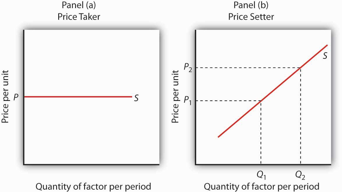
A price-taking firm faces the market-determined price P for the factor in Panel (a) and can purchase any quantity it wants at that price. A price-setting firm faces an upward-sloping supply curve S in Panel (b). The price-setting firm sets the price consistent with the quantity of the factor it wants to obtain. Here, the firm can obtain Q1 units at a price P1, but it must pay a higher price per unit, P2, to obtain Q2 units.
Consider a situation in which one firm is the only buyer of a particular factor. An example might be an isolated mining town where the mine is the single employer. A market in which there is only one buyer of a good, service, or factor of production is called a monopsony. Monopsony is the buyer’s counterpart of monopoly. Monopoly means a single seller; monopsony means a single buyer.
Assume that the suppliers of a factor in a monopsony market are price takers; there is perfect competition in factor supply. But a single firm constitutes the entire market for the factor. That means that the monopsony firm faces the upward-sloping market supply curve for the factor. Such a case is illustrated in Figure 14.2 “Supply and Marginal Factor Cost”, where the price and quantity combinations on the supply curve for the factor are given in the table.
Figure 14.2 Supply and Marginal Factor Cost
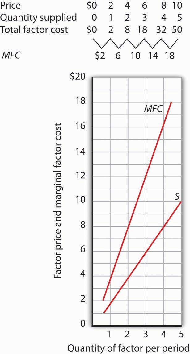
The table gives prices and quantities for the factor supply curve plotted in the graph. Notice that the marginal factor cost curve lies above the supply curve.
Suppose the monopsony firm is now using three units of the factor at a price of $6 per unit. Its total factor cost is $18. Suppose the firm is considering adding one more unit of the factor. Given the supply curve, the only way the firm can obtain four units of the factor rather than three is to offer a higher price of $8 for all four units of the factor. That would increase the firm’s total factor cost from $18 to $32. The marginal factor cost of the fourth unit of the factor is thus $14. It includes the $8 the firm pays for the fourth unit plus an additional $2 for each of the three units the firm was already using, since it has increased the prices for the factor to $8 from $6. The marginal factor cost (MFC) exceeds the price of the factor. We can plot the MFC for each increase in the quantity of the factor the firm uses; notice in Figure 14.2 “Supply and Marginal Factor Cost” that the MFC curve lies above the supply curve. As always in plotting in marginal values, we plot the $14 midway between units three and four because it is the increase in factor cost as the firm goes from three to four units.
Monopsony Equilibrium and the Marginal Decision Rule
The marginal decision rule, as it applies to a firm’s use of factors, calls for the firm to add more units of a factor up to the point that the factor’s MRP is equal to its MFC. Figure 14.3 “Monopsony Equilibrium” illustrates this solution for a firm that is the only buyer of labor in a particular market.
Figure 14.3 Monopsony Equilibrium
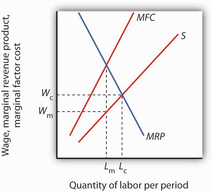
Given the supply curve for labor, S, and the marginal factor cost curve, MFC, the monopsony firm will select the quantity of labor at which the MRP of labor equals its MFC. It thus uses Lm units of labor (determined by at the intersection of MRP and MFC) and pays a wage of Wm per unit (the wage is taken from the supply curve at which Lm units of labor are available). The quantity of labor used by the monopsony firm is less than would be used in a competitive market (Lc); the wage paid, Wm, is lower than would be paid in a competitive labor market.
The firm faces the supply curve for labor, S, and the marginal factor cost curve for labor, MFC. The profit-maximizing quantity is determined by the intersection of the MRP and MFC curves—the firm will hire Lm units of labor. The wage at which the firm can obtain Lm units of labor is given by the supply curve for labor; it is Wm. Labor receives a wage that is less than its MRP.
If the monopsony firm was broken up into a large number of small firms and all other conditions in the market remained unchanged, then the sum of the MRP curves for individual firms would be the market demand for labor. The equilibrium wage would be Wc, and the quantity of labor demanded would be Lc. Thus, compared to a competitive market, a monopsony solution generates a lower factor price and a smaller quantity of the factor demanded.
Monopoly and Monopsony: A Comparison
There is a close relationship between the models of monopoly and monopsony. A clear understanding of this relationship will help to clarify both models.
Figure 14.4 “Monopoly and Monopsony” compares the monopoly and monopsony equilibrium solutions. Both types of firms are price setters: The monopoly is a price setter in its product market; the monopsony is a price setter in its factor market. Both firms must change price to change quantity: The monopoly must lower its product price to sell an additional unit of output, and the monopsony must pay more to hire an additional unit of the factor. Because both types of firms must adjust prices to change quantities, the marginal consequences of their choices are not given by the prices they charge (for products) or pay (for factors). For a monopoly, marginal revenue is less than price; for a monopsony, marginal factor cost is greater than price.
Figure 14.4 Monopoly and Monopsony
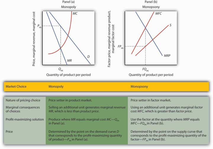
The graphs and the table provide a comparison of monopoly and monopsony.
Both types of firms follow the marginal decision rule: A monopoly produces a quantity of the product at which marginal revenue equals marginal cost; a monopsony employs a quantity of the factor at which marginal revenue product equals marginal factor cost. Both firms set prices at which they can sell or purchase the profit-maximizing quantity. The monopoly sets its product price based on the demand curve it faces; the monopsony sets its factor price based on the factor supply curve it faces.
Monopsony in the Real World
Although cases of pure monopsony are rare, there are many situations in which buyers have a degree of monopsony power. A buyer has monopsony power if it faces an upward-sloping supply curve for a good, service, or factor of production.
For example, a firm that accounts for a large share of employment in a small community may be large enough relative to the labor market that it is not a price taker. Instead, it must raise wages to attract more workers. It thus faces an upward-sloping supply curve and has monopsony power. Because buyers are more likely to have monopsony power in factor markets than in product markets, we shall focus on those.
The next section examines monopsony power in professional sports.
Monopsonies in Sports
Professional sports provide a setting in which economists can test theories of wage determination in competitive versus monopsony labor markets. In their analyses, economists assume professional teams are profit-maximizing firms that hire labor (athletes and other workers) to produce a product: entertainment bought by the fans who watch their games and by other firms that sponsor the games. Fans influence revenues directly by purchasing tickets and indirectly by generating the ratings that determine television and radio advertising revenues from broadcasts of games.
In a competitive system, a player should receive a wage equal to his or her MRP—the increase in team revenues the player is able to produce. As New York Yankees owner George Steinbrenner once put it, “You measure the value of a ballplayer by how many fannies he puts in the seats.”
The monopsony model, however, predicts that players facing monopsony employers will receive wages that are less than their MRPs. A test of monopsony theory, then, would be to determine whether players in competitive markets receive wages equal to their MRPs and whether players in monopsony markets receive less.
Since the late 1970s, there has been a major shift in the rules that govern relations between professional athletes and owners of sports teams. The shift has turned the once monopsonistic market for professional athletes into a competitive one. Before 1977, for example, professional baseball players in the United States played under the terms of the “reserve clause,” which specified that a player was “owned” by his team. Once a team had acquired a player’s contract, the team could sell, trade, retain, or dismiss the player. Unless the team dismissed him, the player was unable to offer his services for competitive bidding by other teams. Moreover, players entered major league baseball through a draft that was structured so that only one team had the right to bid for any one player. Throughout a player’s career, then, there was always only one team that could bid on him—each player faced a monopsony purchaser for his services to major league baseball.
Conditions were similar in other professional sports. Many studies have shown that the salaries of professional athletes in various team sports fell far short of their MRPs while monopsony prevailed.
When the reserve clauses were abandoned, players’ salaries shot up—just as economic theory predicts. Because players could offer their services to other teams, owners began to bid for their services. Profit-maximizing owners were willing to pay athletes their MRPs. Average annual salaries for baseball players rose from about $50,000 in 1975 to nearly $1.4 million in 1997. Average annual player salaries in men’s basketball rose from $109,000 in 1976 to $2.24 million in 1998. Football players worked under an almost pure form of monopsony until 1989, when a few players were allowed free agency status each year. In 1993, when 484 players were released to the market as free agents, those players received pay increases averaging more than 100%. Under the NFL collective bargaining agreement in effect in 1998, players could become unrestricted free agents if they had been playing for four years. There were 305 unrestricted free agents (out of a total player pool of approximately 1,700) that year. About half signed new contracts with their old teams while the other half signed with new teams. Table 14.1 “The Impact of Free Agency” illustrates the impact of free agency in four professional sports.
Table 14.1 The Impact of Free Agency
| Player Salaries As Percentage of Team Revenues | ||||
|---|---|---|---|---|
| MLB | NBA | NFL | NHL | |
| 1970–73 | 15.9 | 46.1 | 34.4 | 21.3 |
| 1998 | 48.4 | 54.2 | 55.4 | 58.4 |
Free agency has increased player share of total revenues in each of the major men’s team sports. Table 14.1 “The Impact of Free Agency” gives player salaries as a percentage of team revenues for major league baseball (MLB), the National Basketball Association (NBA), the National Football League (NFL) and the National Hockey League (NHL) during the 1970–1973 period that players in each league worked under monopsony conditions and in 1998, when players in each league had gained the right of free agency.
Source: Gerald W. Scully, “Player Salary Share and the Distribution of Player Earnings,” Managerial and Decision Economics, 25 (2004): 77–86.
Given the dramatic impact on player salaries of more competitive markets for athletes, events such as the 2004–2005 lockout in hockey came as no surprise. The agreement between the owners of hockey teams and the players in 2005 to limit the total payroll of each team reinstates some of the old monopsony power of the owners. Players had a huge financial stake in resisting such attempts.
Monopsony in Other Labor Markets
A firm that has a dominant position in a local labor market may have monopsony power in that market. Even if a firm does not dominate the total labor market, it may have monopsony power over certain types of labor. For example, a hospital may be the only large employer of nurses in a local market, and it may have monopsony power in employing them.
Colleges and universities generally pay part-time instructors considerably less for teaching a particular course than they pay full-time instructors. In part, the difference reflects the fact that full-time faculty members are expected to have more training and are expected to contribute far more in other areas. But the monopsony model suggests an additional explanation.
Part-time instructors are likely to have other regular employment. A university hiring a local accountant to teach a section of accounting does not have to worry that that person will go to another state to find a better offer as a part-time instructor. For part-time teaching, then, the university may be the only employer in town—and thus able to exert monopsony power to drive the part-time instructor’s wage below the instructor’s MRP.
Monopsony in Other Factor Markets
Monopsony power may also exist in markets for factors other than labor. The military in different countries, for example, has considerable monopsony power in the market for sophisticated military goods. Major retailers often have some monopsony power with respect to some of their suppliers. Sears, for example, is the only wholesale buyer of Craftsman brand tools. One major development in medical care in recent years has been the emergence of managed care organizations that contract with a large number of employers to purchase medical services on behalf of employees. These organizations often have sufficient monopsony power to force down the prices charged by providers such as drug companies, physicians, and hospitals. Countries in which health care is provided by the government, such as Canada and the United Kingdom, are able to exert monopsony power in their purchase of health care services.
Whatever the source of monopsony power, the expected result is the same. Buyers with monopsony power are likely to pay a lower price and to buy a smaller quantity of a particular factor than buyers who operate in a more competitive environment.
Key Takeaways
- In the monopsony model there is one buyer for a good, service, or factor of production. A monopsony firm is a price setter in the market in which it has monopsony power.
- The monopsony buyer selects a profit-maximizing solution by employing the quantity of factor at which marginal factor cost (MFC) equals marginal revenue product (MRP) and paying the price on the factor’s supply curve corresponding to that quantity.
- A degree of monopsony power exists whenever a firm faces an upward-sloping supply curve for a factor.
Try It!
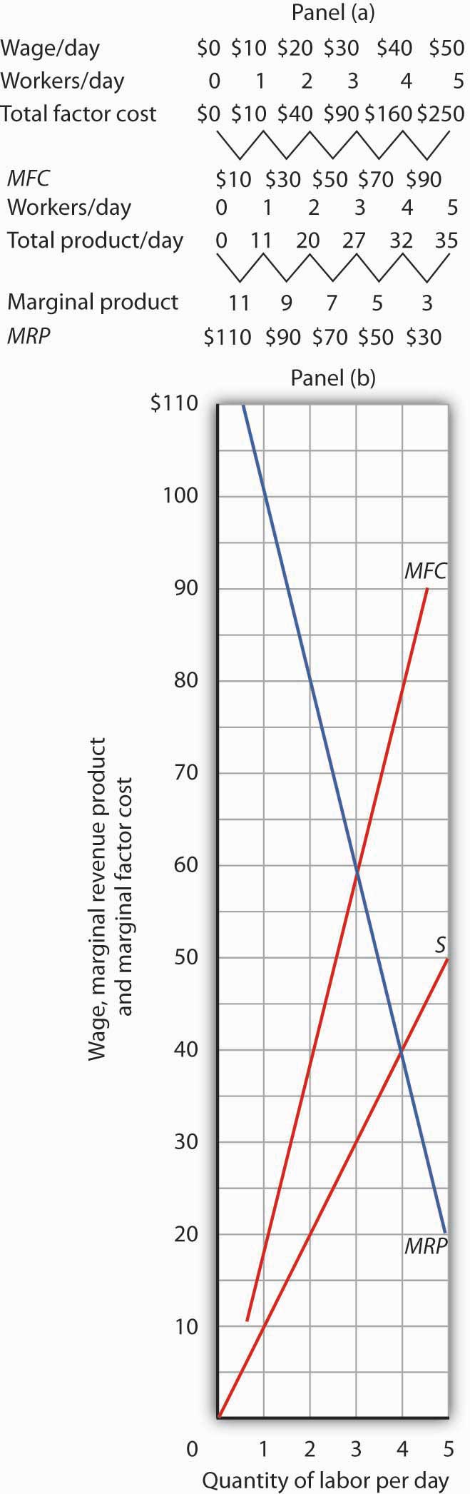
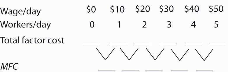
Suppose a firm is the only employer of labor in an isolated area and faces the supply curve for labor suggested by the following table. Plot the supply curve. To compute the marginal factor cost curve, compute total factor cost and then the values for the marginal factor cost curve (remember to plot marginal values at the midpoints of the respective intervals). (Hint: follow the example of Figure 14.2 “Supply and Marginal Factor Cost”.) Compute MRP and plot the MRP curve on the same graph on which you have plotted supply and MFC.
Figure 14.5
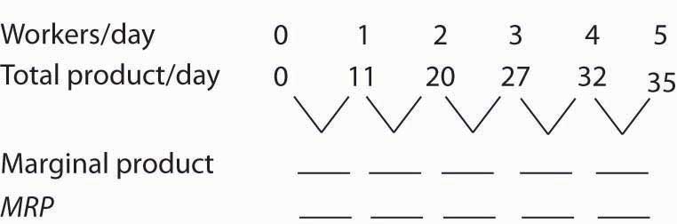
Now suppose you are given the following data for the firm’s total product at each quantity of labor. Compute marginal product. Assume the firm sells its product for $10 per unit in a perfectly competitive market. Compute MRP and plot the MRP curve on the same graph on which you have plotted supply and MFC. Remember to plot marginal values at the midpoints of the respective axes.
Figure 14.6
How much labor will the firm employ? What wage will it pay?
Case in Point: Professional Player Salaries and Monopsony

Professional athletes have not always enjoyed the freedom they have today to seek better offers from other teams. Before 1977, for example, baseball players could deal only with the team that owned their contract—one that “reserved” the player to that team. This reserve clause gave teams monopsony power over the players they employed. Similar restrictions hampered player mobility in men’s football, basketball, and hockey.
Gerald Scully, an economist at the University of Texas at Dallas, estimated the impact of the reserve clause on baseball player salaries. He sought to demonstrate that the player salaries fell short of MRP. Mr. Scully estimated the MRP of players in a two-step process. First, he studied the determinants of team attendance. He found that in addition to factors such as population and income in a team’s home city, the team’s win-loss record had a strong effect on attendance. Second, he examined the player characteristics that determined win-loss records. He found that for hitters, batting average was the variable most closely associated with a team’s winning percentage. For pitchers, it was the earned-run average—the number of earned runs allowed by a pitcher per nine innings pitched.
With equations that predicted a team’s attendance and its win-loss record, Mr. Scully was able to take a particular player, describe him by his statistics, and compute his MRP. Mr. Scully then subtracted costs associated with each player for such things as transportation, lodging, meals, and uniforms to obtain the player’s net MRP. He then compared players’ net MRPs to their salaries.
Mr. Scully’s results, displayed in the table below, show net MRP and salaries, estimated on a career basis, for players he classified as mediocre, average, and star-quality, based on their individual statistics. For average and star-quality players, salaries fell far below net MRP, just as the theory of monopsony suggests.
| Career Net MRP | Career Salary | Salary As % of net MRP | |
|---|---|---|---|
| Hitters | |||
| Mediocre | −$129,300 | $60,800 | |
| Average | 906,700 | 196,200 | 22 |
| Star | 3,139,100 | 477,200 | 15 |
| Pitchers | |||
| Mediocre | −53,600 | 54,800 | |
| Average | 1,119,200 | 222,500 | 20 |
| Star | 3,969,600 | 612,500 | 15 |
The fact that mediocre players with negative net MRPs received salaries presents something of a puzzle. One explanation could be that when they were signed to contracts, these players were expected to perform well, so their salaries reflected their expected contributions to team revenues. Their actual performance fell short, so their wages exceeded their MRPs. Another explanation could be that teams paid young players more than they were expected to contribute to revenues early in their careers in hopes that they would develop into profitable members of the team. In any event, Mr. Scully found that the costs of mediocre players exceeded their estimated contribution to team revenues, giving them negative net MRPs.
In 1977, a lawsuit filed by several baseball players resulted in the partial dismantling of the reserve clause. Players were given the right, after six years with a team, to declare themselves “free agents” and offer their services to other teams. Player salaries quickly rose. The accompanying table shows the pitchers that became free agents in 1977, their estimated net marginal revenue products, and their 1977 salaries. As you can see, salaries for pitchers came quite close to their net MRPs.
| Pitcher | Net MRP | 1977 Salary |
|---|---|---|
| Doyle Alexander | $166,203 | $166,677 |
| Bill Campbell | $205,639 | $210,000 |
| Rollie Fingers | $303,511 | $332,000 |
| Wayne Garland | $282,091 | $230,000 |
| Don Gullett | $340,846 | $349,333 |
The same movement toward giving players greater freedom to deal with other teams occurred in the National Football League (NFL), the National Basketball Association (NBA), and the National Hockey League (NHL). The result in every case was the same: player salaries rose both in absolute terms and as a percentage of total team revenues. Table 14.1 “The Impact of Free Agency” gives player salaries as a percentage of total team revenues in the period 1970–73 and in 1998 for men’s baseball (MLB), basketball, football, and hockey.
The greatest gains came in baseball, which had the most restrictive rules against player movement. Hockey players, too, ended up improving their salaries greatly. By 2004, their salaries totaled 75% of team revenues. The smallest gains came in basketball, where players already had options. The American Basketball Association was formed; it ultimately became part of the National Basketball Association. Basketball players also had the alternative of playing in Europe. But, the economic lesson remains clear: any weakening of the monopsony power of teams results in gains in player salaries.
Sources: Gerald Scully, “Pay and Performance in Major League Baseball,” American Economic Review, 64 (2) (December 1974): 915–30. Gerald W. Scully, “Player Salary Share and the Distribution of Player Earnings,” Managerial and Decision Economics, 25 (2004): 77–86.
Answer to Try It! Problem
The completed tables are shown in Panel (a). Drawing the supply (S), MFC, and MRP curves, we have Panel (b). The monopsony firm will employ three units of labor per day (the quantity at which MRP = MFC) and will pay a wage taken from the supply curve: $30 per day.
Figure 14.8