11.1 Monopolistic Competition: Competition Among Many
Learning Objectives
- Explain the main characteristics of a monopolistically competitive industry, describing both its similarities and differences from the models of perfect competition and monopoly.
- Explain and illustrate both short-run equilibrium and long-run equilibrium for a monopolistically competitive firm.
- Explain what it means to say that a firm operating under monopolistic competition has excess capacity in the long run and discuss the implications of this conclusion.
The first model of an imperfectly competitive industry that we shall investigate has conditions quite similar to those of perfect competition. The model of monopolistic competition assumes a large number of firms. It also assumes easy entry and exit. This model differs from the model of perfect competition in one key respect: it assumes that the goods and services produced by firms are differentiated. This differentiation may occur by virtue of advertising, convenience of location, product quality, reputation of the seller, or other factors. Product differentiation gives firms producing a particular product some degree of price-setting or monopoly power. However, because of the availability of close substitutes, the price-setting power of monopolistically competitive firms is quite limited. Monopolistic competition is a model characterized by many firms producing similar but differentiated products in a market with easy entry and exit.
Restaurants are a monopolistically competitive sector; in most areas there are many firms, each is different, and entry and exit are very easy. Each restaurant has many close substitutes—these may include other restaurants, fast-food outlets, and the deli and frozen-food sections at local supermarkets. Other industries that engage in monopolistic competition include retail stores, barber and beauty shops, auto-repair shops, service stations, banks, and law and accounting firms.
Profit Maximization
Suppose a restaurant raises its prices slightly above those of similar restaurants with which it competes. Will it have any customers? Probably. Because the restaurant is different from other restaurants, some people will continue to patronize it. Within limits, then, the restaurant can set its own prices; it does not take the market prices as given. In fact, differentiated markets imply that the notion of a single “market price” is meaningless.
Because products in a monopolistically competitive industry are differentiated, firms face downward-sloping demand curves. Whenever a firm faces a downward-sloping demand curve, the graphical framework for monopoly can be used. In the short run, the model of monopolistic competition looks exactly like the model of monopoly. An important distinction between monopoly and monopolistic competition, however, emerges from the assumption of easy entry and exit. In monopolistic competition, entry will eliminate any economic profits in the long run. We begin with an analysis of the short run.
The Short Run
Because a monopolistically competitive firm faces a downward-sloping demand curve, its marginal revenue curve is a downward-sloping line that lies below the demand curve, as in the monopoly model. We can thus use the model of monopoly that we have already developed to analyze the choices of a monopsony in the short run.
Figure 11.1 “Short-Run Equilibrium in Monopolistic Competition” shows the demand, marginal revenue, marginal cost, and average total cost curves facing a monopolistically competitive firm, Mama’s Pizza. Mama’s competes with several other similar firms in a market in which entry and exit are relatively easy. Mama’s demand curve D1 is downward-sloping; even if Mama’s raises its prices above those of its competitors, it will still have some customers. Given the downward-sloping demand curve, Mama’s marginal revenue curve MR1 lies below demand. To sell more pizzas, Mama’s must lower its price, and that means its marginal revenue from additional pizzas will be less than price.
Figure 11.1 Short-Run Equilibrium in Monopolistic Competition
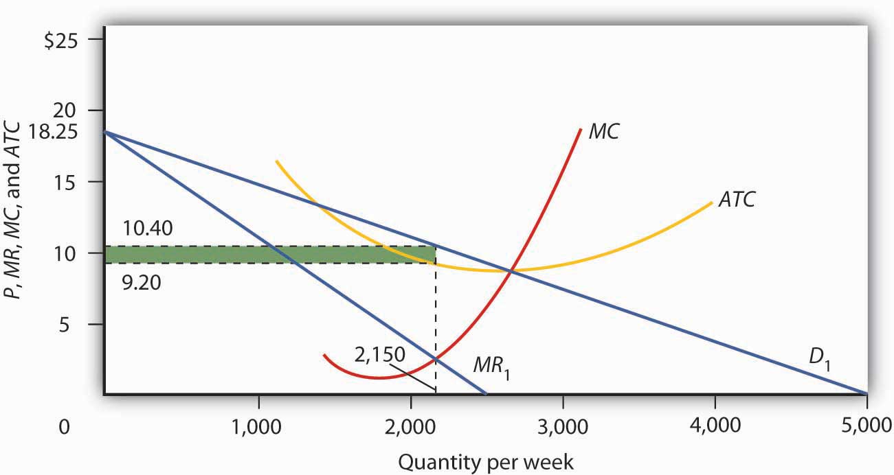
Looking at the intersection of the marginal revenue curve MR1 and the marginal cost curve MC, we see that the profit-maximizing quantity is 2,150 units per week. Reading up to the average total cost curve ATC, we see that the cost per unit equals $9.20. Price, given on the demand curve D1, is $10.40, so the profit per unit is $1.20. Total profit per week equals $1.20 times 2,150, or $2,580; it is shown by the shaded rectangle.
Given the marginal revenue curve MR and marginal cost curve MC, Mama’s will maximize profits by selling 2,150 pizzas per week. Mama’s demand curve tells us that it can sell that quantity at a price of $10.40. Looking at the average total cost curve ATC, we see that the firm’s cost per unit is $9.20. Its economic profit per unit is thus $1.20. Total economic profit, shown by the shaded rectangle, is $2,580 per week.
The Long Run
We see in Figure 11.1 “Short-Run Equilibrium in Monopolistic Competition” that Mama’s Pizza is earning an economic profit. If Mama’s experience is typical, then other firms in the market are also earning returns that exceed what their owners could be earning in some related activity. Positive economic profits will encourage new firms to enter Mama’s market.
As new firms enter, the availability of substitutes for Mama’s pizzas will increase, which will reduce the demand facing Mama’s Pizza and make the demand curve for Mama’s Pizza more elastic. Its demand curve will shift to the left. Any shift in a demand curve shifts the marginal revenue curve as well. New firms will continue to enter, shifting the demand curves for existing firms to the left, until pizza firms such as Mama’s no longer make an economic profit. The zero-profit solution occurs where Mama’s demand curve is tangent to its average total cost curve—at point A in Figure 11.2 “Monopolistic Competition in the Long Run”. Mama’s price will fall to $10 per pizza and its output will fall to 2,000 pizzas per week. Mama’s will just cover its opportunity costs, and thus earn zero economic profit. At any other price, the firm’s cost per unit would be greater than the price at which a pizza could be sold, and the firm would sustain an economic loss. Thus, the firm and the industry are in long-run equilibrium. There is no incentive for firms to either enter or leave the industry.
Figure 11.2 Monopolistic Competition in the Long Run
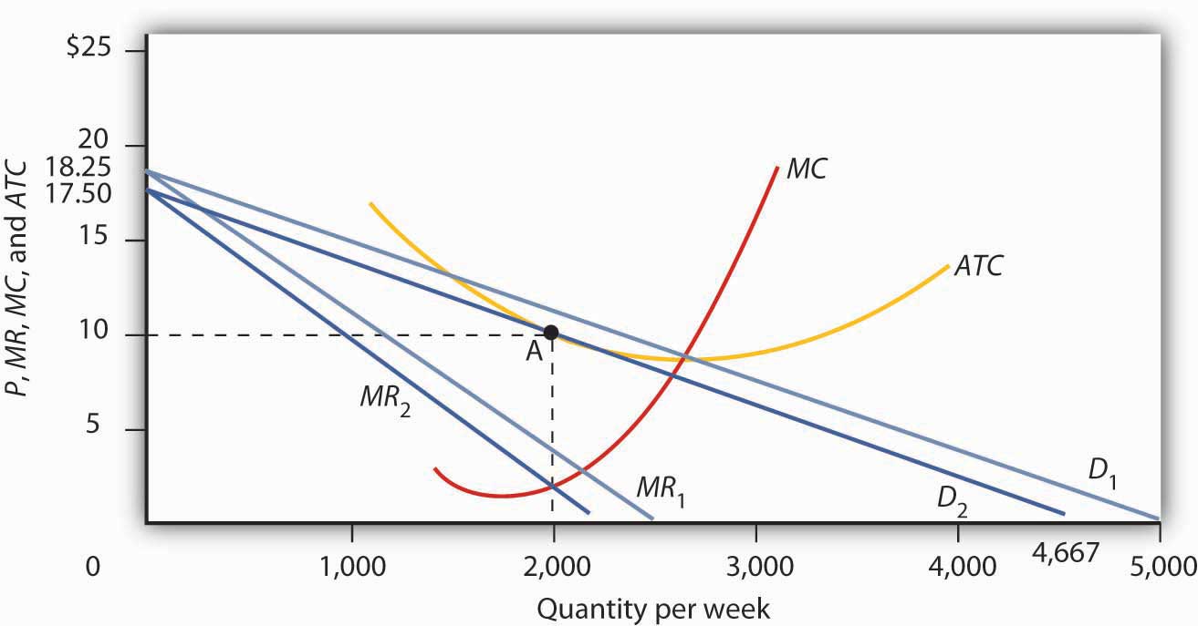
The existence of economic profits in a monopolistically competitive industry will induce entry in the long run. As new firms enter, the demand curve D1 and marginal revenue curve MR1 facing a typical firm will shift to the left, to D2 and MR2. Eventually, this shift produces a profit-maximizing solution at zero economic profit, where D2 is tangent to the average total cost curve ATC (point A). The long-run equilibrium solution here is an output of 2,000 units per week at a price of $10 per unit.
Had Mama’s Pizza and other similar restaurants been incurring economic losses, the process of moving to long-run equilibrium would work in reverse. Some firms would exit. With fewer substitutes available, the demand curve faced by each remaining firm would shift to the right. Price and output at each restaurant would rise. Exit would continue until the industry was in long-run equilibrium, with the typical firm earning zero economic profit.
Such comings and goings are typical of monopolistic competition. Because entry and exit are easy, favorable economic conditions in the industry encourage start-ups. New firms hope that they can differentiate their products enough to make a go of it. Some will; others will not. Competitors to Mama’s may try to improve the ambience, play different music, offer pizzas of different sizes and types. It might take a while for other restaurants to come up with just the right product to pull customers and profits away from Mama’s. But as long as Mama’s continues to earn economic profits, there will be incentives for other firms to try.
Heads Up!
The term “monopolistic competition” is easy to confuse with the term “monopoly.” Remember, however, that the two models are characterized by quite different market conditions. A monopoly is a single firm with high barriers to entry. Monopolistic competition implies an industry with many firms, differentiated products, and easy entry and exit.
Why is the term monopolistic competition used to describe this type of market structure? The reason is that it bears some similarities to both perfect competition and to monopoly. Monopolistic competition is similar to perfect competition in that in both of these market structures many firms make up the industry and entry and exit are fairly easy. Monopolistic competition is similar to monopoly in that, like monopoly firms, monopolistically competitive firms have at least some discretion when it comes to setting prices. However, because monopolistically competitive firms produce goods that are close substitutes for those of rival firms, the degree of monopoly power that monopolistically competitive firms possess is very low.
Excess Capacity: The Price of Variety
The long-run equilibrium solution in monopolistic competition always produces zero economic profit at a point to the left of the minimum of the average total cost curve. That is because the zero profit solution occurs at the point where the downward-sloping demand curve is tangent to the average total cost curve, and thus the average total cost curve is itself downward-sloping. By expanding output, the firm could lower average total cost. The firm thus produces less than the output at which it would minimize average total cost. A firm that operates to the left of the lowest point on its average total cost curve has excess capacity.
Because monopolistically competitive firms charge prices that exceed marginal cost, monopolistic competition is inefficient. The marginal benefit consumers receive from an additional unit of the good is given by its price. Since the benefit of an additional unit of output is greater than the marginal cost, consumers would be better off if output were expanded. Furthermore, an expansion of output would reduce average total cost. But monopolistically competitive firms will not voluntarily increase output, since for them, the marginal revenue would be less than the marginal cost.
One can thus criticize a monopolistically competitive industry for falling short of the efficiency standards of perfect competition. But monopolistic competition is inefficient because of product differentiation. Think about a monopolistically competitive activity in your area. Would consumers be better off if all the firms in this industry produced identical products so that they could match the assumptions of perfect competition? If identical products were impossible, would consumers be better off if some of the firms were ordered to shut down on grounds the model predicts there will be “too many” firms? The inefficiency of monopolistic competition may be a small price to pay for a wide range of product choices. Furthermore, remember that perfect competition is merely a model. It is not a goal toward which an economy might strive as an alternative to monopolistic competition.
Key Takeaways
- A monopolistically competitive industry features some of the same characteristics as perfect competition: a large number of firms and easy entry and exit.
- The characteristic that distinguishes monopolistic competition from perfect competition is differentiated products; each firm is a price setter and thus faces a downward-sloping demand curve.
- Short-run equilibrium for a monopolistically competitive firm is identical to that of a monopoly firm. The firm produces an output at which marginal revenue equals marginal cost and sets its price according to its demand curve.
- In the long run in monopolistic competition any economic profits or losses will be eliminated by entry or by exit, leaving firms with zero economic profit.
- A monopolistically competitive industry will have some excess capacity; this may be viewed as the cost of the product diversity that this market structure produces.
Try It!
Suppose the monopolistically competitive restaurant industry in your town is in long-run equilibrium, when difficulties in hiring cause restaurants to offer higher wages to cooks, servers, and dishwashers. Using graphs similar to Figure 11.1 “Short-Run Equilibrium in Monopolistic Competition” and Figure 11.2 “Monopolistic Competition in the Long Run”, explain the effect of the wage increase on the industry in the short run and in the long run. Be sure to include in your answer an explanation of what happens to price, output, and economic profit.
Case in Point: Craft Brewers: The Rebirth of a Monopolistically Competitive Industry
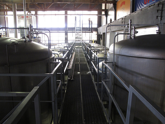
In the early 1900s, there were about 2,000 local beer breweries across America. Prohibition in the 1920s squashed the industry; after the repeal of Prohibition, economies of scale eliminated smaller breweries. By the early 1980s only about 40 remained in existence.
But the American desire for more variety has led to the rebirth of the nearly defunct industry. To be sure, large, national beer companies dominated the overall ale market in 1980 and they still do today, with 43 large national and regional breweries sharing about 85% of the U.S. market for beer. But their emphasis on similarly tasting, light lagers (at least, until they felt threatened enough by the new craft brewers to come up with their own specialty brands) left many niches to be filled. One niche was filled by imports, accounting for about 12% of the U.S. market. That leaves 3 to 4% of the national market for the domestic specialty or “craft” brewers.
The new craft brewers, which include contract brewers, regional specialty brewers, microbreweries, and brewpubs, offer choice. As Neal Leathers at Big Sky Brewing Company in Missoula, Montana put it, “We sort of convert people. If you haven’t had very many choices, and all of a sudden you get choices—especially if those choices involve a lot of flavor and quality—it’s hard to go back.”
Aided by the recent legalization in most states of brewpubs, establishments where beers are manufactured and retailed on the same premises, the number of microbreweries grew substantially over the last 25 years. A recent telephone book in Colorado Springs, a city with a population of about a half million and the home of the authors of your textbook, listed nine microbreweries and brewpubs; more exist, but prefer to be listed as restaurants.
To what extent does this industry conform to the model of monopolistic competition? Clearly, the microbreweries sell differentiated products, giving them some degree of price-setting power. A sample of four brewpubs in the downtown area of Colorado Springs revealed that the price of a house beer ranged from 13 to 22 cents per ounce.
Entry into the industry seems fairly easy, judging from the phenomenal growth of the industry. After more than a decade of explosive growth and then a period of leveling off, the number of craft breweries, as they are referred to by the Association of Brewers, stood at 1,463 in 2007. The start-up cost ranges from $100,000 to $400,000, according to Kevin Head, the owner of the Rhino Bar, also in Missoula.
The monopolistically competitive model also predicts that while firms can earn positive economic profits in the short run, entry of new firms will shift the demand curve facing each firm to the left and economic profits will fall toward zero. Some firms will exit as competitors win customers away from them. In the combined microbrewery and brewpub sub-sectors of the craft beer industry in 2007, for example, there were 94 openings and 51 closings.
Sources: Jim Ludwick, “The Art of Zymurgy—It’s the Latest Thing: Microbrewers are Tapping into the New Specialty Beer Market,” Missoulian (November 29, 1996): p. A1; Brewers Association, “2007 Craft Beer Industry Statistics,” April 17, 2008, www.beertown.org/craftbrewing/statistics.html.
Answer to Try It! Problem
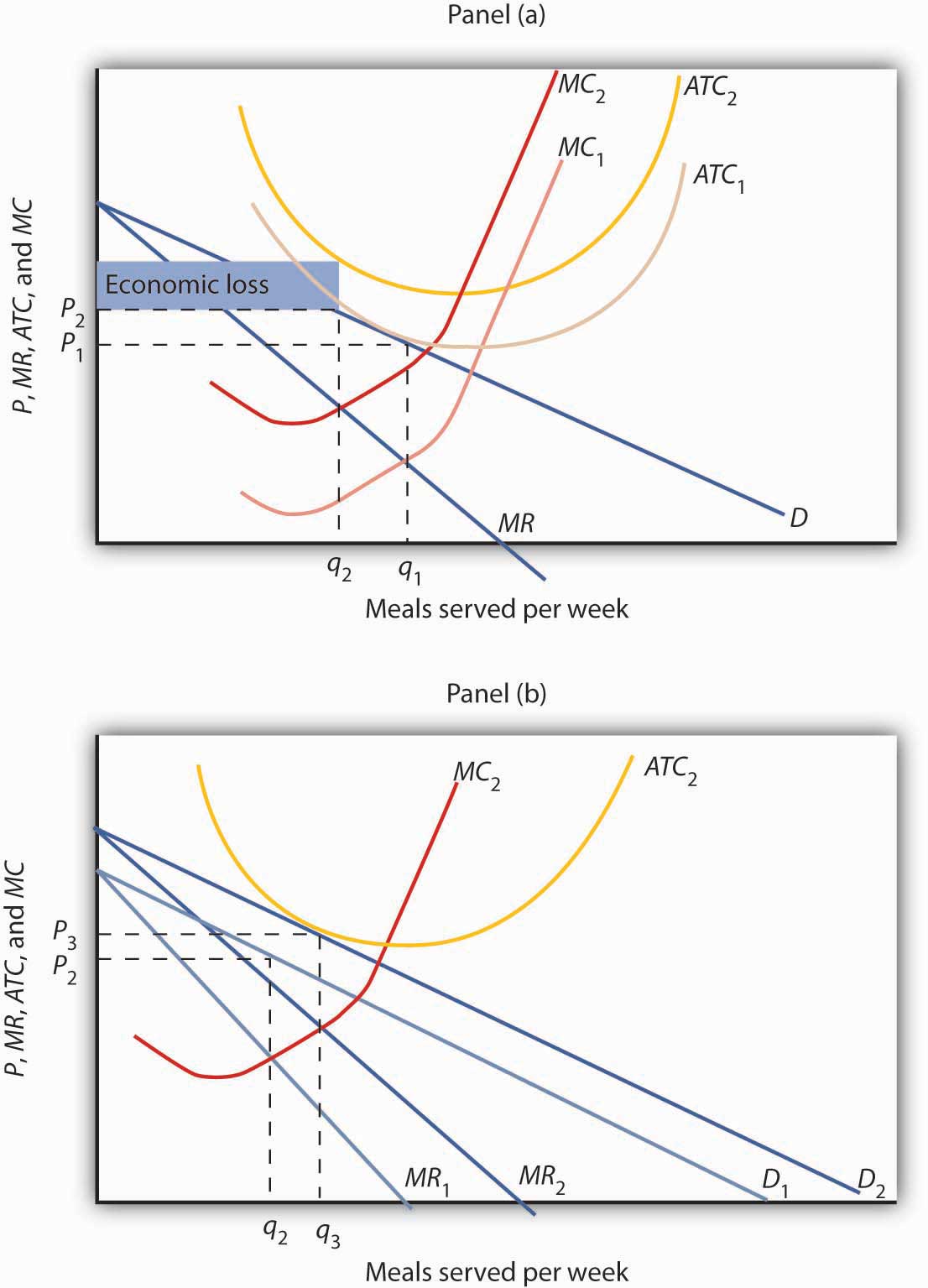
As shown in Panel (a), higher wages would cause both MC and ATC to increase. The upward shift in MC from MC1 to MC2 would cause the profit-maximizing level of output (number of meals served per week, in this case) to fall from q1 to q2 and price to increase from P1 to P2. The increase in ATC from ATC1 to ATC2 would mean that some restaurants would be earning negative economic profits, as shown by the shaded area.
As shown in Panel (b), in the long run, as some restaurants close down, the demand curve faced by the typical remaining restaurant would shift to the right from D1 to D2. The demand curve shift leads to a corresponding shift in marginal revenue from MR1 to MR2. Price would increase further from P2 to P3, and output would increase to q3, above q2. In the new long-run equilibrium, restaurants would again be earning zero economic profit.
Figure 11.4