5.3 Price Elasticity of Supply
Learning Objectives
- Explain the concept of elasticity of supply and its calculation.
- Explain what it means for supply to be price inelastic, unit price elastic, price elastic, perfectly price inelastic, and perfectly price elastic.
- Explain why time is an important determinant of price elasticity of supply.
- Apply the concept of price elasticity of supply to the labor supply curve.
The elasticity measures encountered so far in this chapter all relate to the demand side of the market. It is also useful to know how responsive quantity supplied is to a change in price.
Suppose the demand for apartments rises. There will be a shortage of apartments at the old level of apartment rents and pressure on rents to rise. All other things unchanged, the more responsive the quantity of apartments supplied is to changes in monthly rents, the lower the increase in rent required to eliminate the shortage and to bring the market back to equilibrium. Conversely, if quantity supplied is less responsive to price changes, price will have to rise more to eliminate a shortage caused by an increase in demand.
This is illustrated in Figure 5.10 “Increase in Apartment Rents Depends on How Responsive Supply Is”. Suppose the rent for a typical apartment had been R0 and the quantity Q0 when the demand curve was D1 and the supply curve was either S1 (a supply curve in which quantity supplied is less responsive to price changes) or S2 (a supply curve in which quantity supplied is more responsive to price changes). Note that with either supply curve, equilibrium price and quantity are initially the same. Now suppose that demand increases to D2, perhaps due to population growth. With supply curve S1, the price (rent in this case) will rise to R1 and the quantity of apartments will rise to Q1. If, however, the supply curve had been S2, the rent would only have to rise to R2 to bring the market back to equilibrium. In addition, the new equilibrium number of apartments would be higher at Q2. Supply curve S2 shows greater responsiveness of quantity supplied to price change than does supply curve S1.
Figure 5.10 Increase in Apartment Rents Depends on How Responsive Supply Is
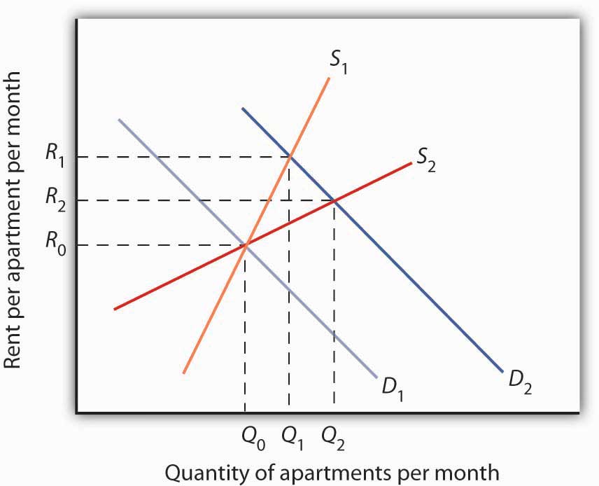
The more responsive the supply of apartments is to changes in price (rent in this case), the less rents rise when the demand for apartments increases.
We measure the price elasticity of supply (eS) as the ratio of the percentage change in quantity supplied of a good or service to the percentage change in its price, all other things unchanged:
Equation 5.6
[latex]e_S = \frac{ \% \: change \: in \: quantity \: supplied}{ \% \: change \: in \: price}[/latex]
Because price and quantity supplied usually move in the same direction, the price elasticity of supply is usually positive. The larger the price elasticity of supply, the more responsive the firms that supply the good or service are to a price change.
Supply is price elastic if the price elasticity of supply is greater than 1, unit price elastic if it is equal to 1, and price inelastic if it is less than 1. A vertical supply curve, as shown in Panel (a) of Figure 5.11 “Supply Curves and Their Price Elasticities”, is perfectly inelastic; its price elasticity of supply is zero. The supply of Beatles’ songs is perfectly inelastic because the band no longer exists. A horizontal supply curve, as shown in Panel (b) of Figure 5.11 “Supply Curves and Their Price Elasticities”, is perfectly elastic; its price elasticity of supply is infinite. It means that suppliers are willing to supply any amount at a certain price.
Figure 5.11 Supply Curves and Their Price Elasticities
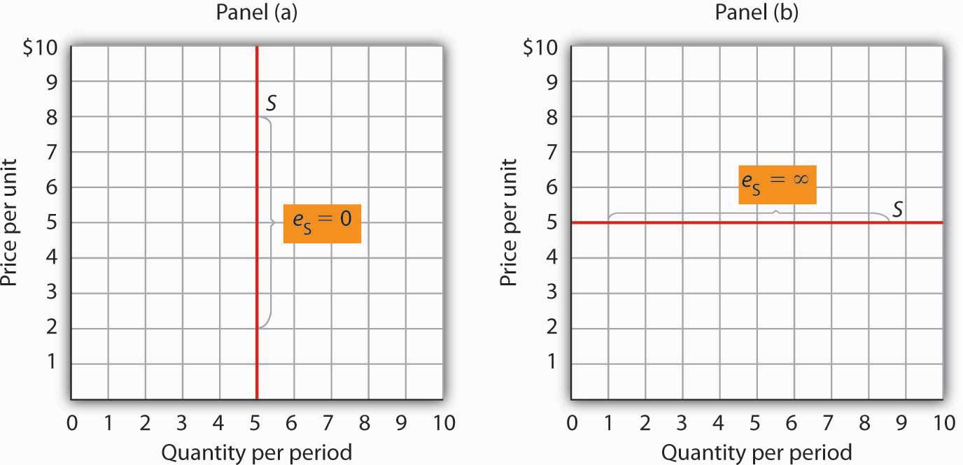
The supply curve in Panel (a) is perfectly inelastic. In Panel (b), the supply curve is perfectly elastic.
Time: An Important Determinant of the Elasticity of Supply
Time plays a very important role in the determination of the price elasticity of supply. Look again at the effect of rent increases on the supply of apartments. Suppose apartment rents in a city rise. If we are looking at a supply curve of apartments over a period of a few months, the rent increase is likely to induce apartment owners to rent out a relatively small number of additional apartments. With the higher rents, apartment owners may be more vigorous in reducing their vacancy rates, and, indeed, with more people looking for apartments to rent, this should be fairly easy to accomplish. Attics and basements are easy to renovate and rent out as additional units. In a short period of time, however, the supply response is likely to be fairly modest, implying that the price elasticity of supply is fairly low. A supply curve corresponding to a short period of time would look like S1 in Figure 5.10 “Increase in Apartment Rents Depends on How Responsive Supply Is”. It is during such periods that there may be calls for rent controls.
If the period of time under consideration is a few years rather than a few months, the supply curve is likely to be much more price elastic. Over time, buildings can be converted from other uses and new apartment complexes can be built. A supply curve corresponding to a longer period of time would look like S2 in Figure 5.10 “Increase in Apartment Rents Depends on How Responsive Supply Is”.
Elasticity of Labor Supply: A Special Application
The concept of price elasticity of supply can be applied to labor to show how the quantity of labor supplied responds to changes in wages or salaries. What makes this case interesting is that it has sometimes been found that the measured elasticity is negative, that is, that an increase in the wage rate is associated with a reduction in the quantity of labor supplied.
In most cases, labor supply curves have their normal upward slope: higher wages induce people to work more. For them, having the additional income from working more is preferable to having more leisure time. However, wage increases may lead some people in very highly paid jobs to cut back on the number of hours they work because their incomes are already high and they would rather have more time for leisure activities. In this case, the labor supply curve would have a negative slope. The reasons for this phenomenon are explained more fully in a later chapter.
This chapter has covered a variety of elasticity measures. All report the degree to which a dependent variable responds to a change in an independent variable. As we have seen, the degree of this response can play a critically important role in determining the outcomes of a wide range of economic events. Table 5.2 “Selected Elasticity Estimates”1 provides examples of some estimates of elasticities.
Table 5.2 Selected Elasticity Estimates
| Product | Elasticity | Product | Elasticity | Product | Elasticity |
|---|---|---|---|---|---|
| Price Elasticity of Demand | Cross Price Elasticity of Demand | Income Elasticity of Demand | |||
| Crude oil (U.S.)* | −0.06 | Alcohol with respect to price of heroin | −0.05 | Speeding citations | −0.26 to −0.33 |
| Gasoline | −0.1 | Fuel with respect to price of transport | −0.48 | Urban Public Trust in France and Madrid (respectively) | −0.23; −0.26 |
| Speeding citations | −0.21 | Alcohol with respect to price of food | −0.16 | Ground beef | −0.197 |
| Cabbage | −0.25 | Marijuana with respect to price of heroin (similar for cocaine) | −0.01 | Lottery instant game sales in Colorado | −0.06 |
| Cocaine (two estimates) | −0.28; −1.0 | Beer with respect to price of wine distilled liquor (young drinkers) | 0.0 | Heroin | −0.00 |
| Alcohol | −0.30 | Beer with respect to price of distilled liquor (young drinkers) | 0.0 | Marijuana, alcohol, cocaine | +0.00 |
| Peaches | −0.38 | Pork with respect to price of poultry | 0.06 | Potatoes | 0.15 |
| Marijuana | −0.4 | Pork with respect to price of ground beef | 0.23 | Food** | 0.2 |
| Cigarettes (all smokers; two estimates) | −0.4; −0.32 | Ground beef with respect to price of poultry | 0.24 | Clothing*** | 0.3 |
| Crude oil (U.S.)** | −0.45 | Ground beef with respect to price of pork | 0.35 | Beer | 0.4 |
| Milk (two estimates) | −0.49; −0.63 | Coke with respect to price of Pepsi | 0.61 | Eggs | 0.57 |
| Gasoline (intermediate term) | −0.5 | Pepsi with respect to price of Coke | 0.80 | Coke | 0.60 |
| Soft drinks | −0.55 | Local television advertising with respect to price of radio advertising | 1.0 | Shelter** | 0.7 |
| Transportation* | −0.6 | Smokeless tobacco with respect to price of cigarettes (young males) | 1.2 | Beef (table cuts—not ground) | 0.81 |
| Food | −0.7 | Price Elasticity of Supply | Oranges | 0.83 | |
| Beer | −0.7 to −0.9 | Physicians (Specialist) | −0.3 | Apples | 1.32 |
| Cigarettes (teenagers; two estimates) | −0.9 to −1.5 | Physicians (Primary Care) | 0.0 | Leisure** | 1.4 |
| Heroin | −0.94 | Physicians (Young male) | 0.2 | Peaches | 1.43 |
| Ground beef | −1.0 | Physicians (Young female) | 0.5 | Health care** | 1.6 |
| Cottage cheese | −1.1 | Milk* | 0.36 | Higher education | 1.67 |
| Gasoline** | −1.5 | Milk** | 0.5 | ||
| Coke | −1.71 | Child care labor | 2 | ||
| Transportation | −1.9 | ||||
| Pepsi | −2.08 | ||||
| Fresh tomatoes | −2.22 | ||||
| Food** | −2.3 | ||||
| Lettuce | −2.58 | ||||
| Note: *=short-run; **=long-run | |||||
Key Takeaways
- The price elasticity of supply measures the responsiveness of quantity supplied to changes in price. It is the percentage change in quantity supplied divided by the percentage change in price. It is usually positive.
- Supply is price inelastic if the price elasticity of supply is less than 1; it is unit price elastic if the price elasticity of supply is equal to 1; and it is price elastic if the price elasticity of supply is greater than 1. A vertical supply curve is said to be perfectly inelastic. A horizontal supply curve is said to be perfectly elastic.
- The price elasticity of supply is greater when the length of time under consideration is longer because over time producers have more options for adjusting to the change in price.
- When applied to labor supply, the price elasticity of supply is usually positive but can be negative. If higher wages induce people to work more, the labor supply curve is upward sloping and the price elasticity of supply is positive. In some very high-paying professions, the labor supply curve may have a negative slope, which leads to a negative price elasticity of supply.
Try It!
In the late 1990s, it was reported on the news that the high-tech industry was worried about being able to find enough workers with computer-related expertise. Job offers for recent college graduates with degrees in computer science went with high salaries. It was also reported that more undergraduates than ever were majoring in computer science. Compare the price elasticity of supply of computer scientists at that point in time to the price elasticity of supply of computer scientists over a longer period of, say, 1999 to 2009.
Case in Point: A Variety of Labor Supply Elasticities

Studies support the idea that labor supply is less elastic in high-paying jobs than in lower-paying ones.
For example, David M. Blau estimated the labor supply of child-care workers to be very price elastic, with estimated price elasticity of labor supply of about 2.0. This means that a 10% increase in wages leads to a 20% increase in the quantity of labor supplied. John Burkett estimated the labor supply of both nursing assistants and nurses to be price elastic, with that of nursing assistants to be 1.9 (very close to that of child-care workers) and of nurses to be 1.1. Note that the price elasticity of labor supply of the higher-paid nurses is a bit lower than that of lower-paid nursing assistants.
In contrast, John Rizzo and David Blumenthal estimated the price elasticity of labor supply for young physicians (under the age of 40) to be about 0.3. This means that a 10% increase in wages leads to an increase in the quantity of labor supplied of only about 3%. In addition, when Rizzo and Blumenthal looked at labor supply elasticities by gender, they found the female physicians’ labor supply price elasticity to be a bit higher (at about 0.5) than that of the males (at about 0.2) in the sample. Because earnings of female physicians in the sample were lower than earnings of the male physicians in the sample, this difference in labor supply elasticities was expected. Moreover, since the sample consisted of physicians in the early phases of their careers, the positive, though small, price elasticities were also expected. Many of the individuals in the sample also had high debt levels, often from educational loans. Thus, the chance to earn more by working more is an opportunity to repay educational and other loans.
In another study of physicians’ labor supply that was not restricted to young physicians, Douglas M. Brown found the labor supply price elasticity for primary care physicians to be close to zero and that of specialists to be negative, at about −0.3. Thus, for this sample of physicians, increases in wages have little or no effect on the amount the primary care doctors work, while a 10% increase in wages for specialists reduces their quantity of labor supplied by about 3%. Because the earnings of specialists exceed those of primary care doctors, this elasticity differential also makes sense.
Sources: David M. Blau, “The Supply of Child Care Labor,” Journal of Labor Economics 11:2 (April 1993): 324–347; David M. Brown, “The Rising Cost of Physician’s Services: A Correction and Extension on Supply,” Review of Economics and Statistics 76 (2) (May 1994): 389–393; John P. Burkett, “The Labor Supply of Nurses and Nursing Assistants in the United States,” Eastern Economic Journal 31(4) (Fall 2005): 585–599; John A. Rizzo and Paul Blumenthal. “Physician Labor Supply: Do Income Effects Matter?” Journal of Health Economics 13:4 (December 1994): 433–453.
Answer to Try It! Problem
While at a point in time the supply of people with degrees in computer science is very price inelastic, over time the elasticity should rise. That more students were majoring in computer science lends credence to this prediction. As supply becomes more price elastic, salaries in this field should rise more slowly.
1Although close to zero in all cases, the significant and positive signs of income elasticity for marijuana, alcohol, and cocaine suggest that they are normal goods, but significant and negative signs, in the case of heroin, suggest that heroin is an inferior good. Saffer and Chaloupka (cited below) suggest the effects of income for all four substances might be affected by education. [Other References listed below]
References
Adesoji, O. Adelaja, A. “Price Changes, Supply Elasticities, Industry Organization, and Dairy Output Distribution,” American Journal of Agricultural Economics 73:1 (February 1991):89–102.
Bar-Ilan, A., and Bruce Sacerdote, “The Response of Criminals and Non-Criminals to Fines,” Journal of Law and Economics, 47:1 (April 2004): 1–17.
Baye, M.R., D.W. Jansen, and J.W. Lee, “Advertising Effects in Complete Demand Systems,” Applied Economics 24 (1992):1087–1096.
Bhuyan, S., and Rigoberto A. Lopez, “Oligopoly Power in the Food and Tobacco Industries,” American Journal of Agricultural Economics 79 (August 1997):1035–1043.
Blau, D. M., “The Supply of Child Care Labor,” Journal of Labor Economics 2(11) (April 1993):324–347.
Blundell, R., et al., “What Do We Learn About Consumer Demand Patterns from Micro Data?”, American Economic Review 83(3) (June 1993):570–597.
Bresson, G., Joyce Dargay, Jean-Loup Madre, and Alain Pirotte, “Economic and Structural Determinants of the Demand for French Transport: An Analysis on a Panel of French Urban Areas Using Shrinkage Estimators,” Transportation Research: Part A 38:4 (May 2004): 269–285.
Brester, G. W., and Michael K. Wohlgenant, “Estimating Interrelated Demands for Meats Using New Measures for Ground and Table Cut Beef,” American Journal of Agricultural Economics 73 (November 1991):1182–1194.
Brown, D. M., “The Rising Price of Physicians’ Services: A Correction and Extension on Supply,” Review of Economics and Statistics 76(2) (May 1994):389–393.
Davis, G. C., and Michael K. Wohlgenant, “Demand Elasticities from a Discrete Choice Model: The Natural Christmas Tree Market,” Journal of Agricultural Economics 75(3) (August 1993):730–738.
Ekelund, R. B., S. Ford, and John D. Jackson. “Are Local TV Markets Separate Markets?” International Journal of the Economics of Business 7:1 (2000): 79–97.
Elzinga, K. G., “Beer,” in Walter Adams and James Brock, eds., The Structure of American Industry, 9th ed. (Englewood Cliffs: Prentice Hall, 1995), pp. 119–151.
Farrelly, M. C., Terry F. Pechacek, and Frank J. Chaloupka; “The Impact of Tobacco Control Program Expenditures on Aggregate Cigarette Sales: 1981–2000,” Journal of Health Economics 22:5 (September 2003): 843–859.
Fogel, R. W., “Catching Up With the Economy,” American Economic Review 89(1) (March, 1999):1–21.
Gasmi, F., et al., “Econometric Analysis of Collusive Behavior in a Soft-Drink Market,” Journal of Economics and Management Strategy (Summer 1992), pp. 277–311.
Griffin, J. M., and Henry B. Steele, Energy Economics and Policy (New York: Academic Press, 1980), p. 232.
Grossman, M., “A Survey of Economic Models of Addictive Behavior,” Journal of Drug Issues 28:3 (Summer 1998):631–643.
Grossman, M., “Cigarette Taxes,” Public Health Reports 112:4 (July/August 1997): 290–297.
Grossman, M., and Henry Saffer, “Beer Taxes, the Legal Drinking Age, and Youth Motor Vehicle Fatalities,” Journal of Legal Studies 16(2) (June 1987):351–374.
Hansen, A., “The Tax Incidence of the Colorado State Lottery Instant Game,” Public Finance Quarterly 23(3) (July, 1995):385–398.
Heien, D., and Cathy Roheim Wessells, “The Demand for Dairy Products: Structure, Prediction, and Decomposition,” American Journal of Agriculture Economics (May 1988):219–228.
Kleinman, M. A. R., Marijuana: Costs of Abuse, Costs of Control (NY:Greenwood Press, 1989).
Levine, J. M., et al., “The Demand for Higher Education in Three Mid-Atlantic States,” New York Economic Review 18 (Fall 1988):3–20.
Matas, A., “Demand and Revenue Implications of an Integrated Transport Policy: The Case of Madrid,” Transport Reviews, 24:2 (March 2004): 195–217.
Rizzo J. A., and David Blumenthal, “Physician Labor Supply: Do Income Effects Matter?” Journal of Health Economics 13(4) (December 1994):433–453.
Ross, H., and Frank J. Chaloupka, “The Effect of Public Policies and Prices on Youth Smoking,” Southern Economic Journal 70:4 (April 2004): 796–815.
Saffer, H., and Frank Chaloupka, “The Demand for Illicit Drugs,” Economic Inquiry 37(3) (July, 1999): 401–411.
Suits, D. B., “Agriculture,” in Walter Adams and James Brock, eds., The Structure of American Industry, 9th ed. (Englewood Cliffs: Prentice Hall, , 1995), pp. 1–33.
Tauras. J. A., “Public Policy and Smoking Cessation among Young Adults in the United States,” Health Policy, 68:3 (June 2004): 321–332.
