22.1 Aggregate Demand
Learning Objectives
- Define potential output, also called the natural level of GDP.
- Define aggregate demand, represent it using a hypothetical aggregate demand curve, and identify and explain the three effects that cause this curve to slope downward.
- Distinguish between a change in the aggregate quantity of goods and services demanded and a change in aggregate demand.
- Use examples to explain how each component of aggregate demand can be a possible aggregate demand shifter.
- Explain what a multiplier is and tell how to calculate it.
Firms face four sources of demand: households (personal consumption), other firms (investment), government agencies (government purchases), and foreign markets (net exports). Aggregate demand is the relationship between the total quantity of goods and services demanded (from all the four sources of demand) and the price level, all other determinants of spending unchanged. The aggregate demand curve is a graphical representation of aggregate demand.
The Slope of the Aggregate Demand Curve
We will use the implicit price deflator as our measure of the price level; the aggregate quantity of goods and services demanded is measured as real GDP. The table in Figure 22.1 “Aggregate Demand” gives values for each component of aggregate demand at each price level for a hypothetical economy. Various points on the aggregate demand curve are found by adding the values of these components at different price levels. The aggregate demand curve for the data given in the table is plotted on the graph in Figure 22.1 “Aggregate Demand”. At point A, at a price level of 1.18, $11,800 billion worth of goods and services will be demanded; at point C, a reduction in the price level to 1.14 increases the quantity of goods and services demanded to $12,000 billion; and at point E, at a price level of 1.10, $12,200 billion will be demanded.
Figure 22.1 Aggregate Demand
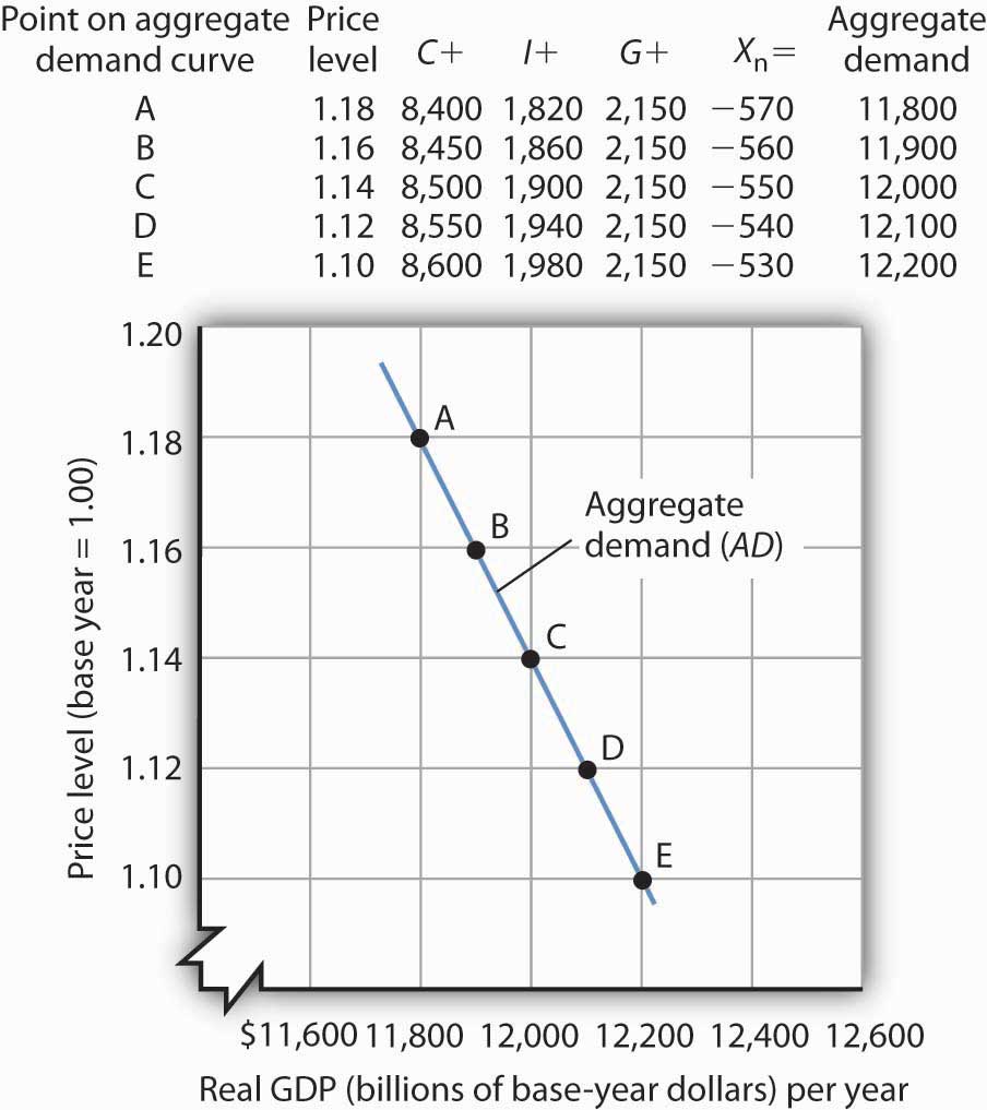
An aggregate demand curve (AD) shows the relationship between the total quantity of output demanded (measured as real GDP) and the price level (measured as the implicit price deflator). At each price level, the total quantity of goods and services demanded is the sum of the components of real GDP, as shown in the table. There is a negative relationship between the price level and the total quantity of goods and services demanded, all other things unchanged.
The negative slope of the aggregate demand curve suggests that it behaves in the same manner as an ordinary demand curve. But we cannot apply the reasoning we use to explain downward-sloping demand curves in individual markets to explain the downward-sloping aggregate demand curve. There are two reasons for a negative relationship between price and quantity demanded in individual markets. First, a lower price induces people to substitute more of the good whose price has fallen for other goods, increasing the quantity demanded. Second, the lower price creates a higher real income. This normally increases quantity demanded further.
Neither of these effects is relevant to a change in prices in the aggregate. When we are dealing with the average of all prices—the price level—we can no longer say that a fall in prices will induce a change in relative prices that will lead consumers to buy more of the goods and services whose prices have fallen and less of the goods and services whose prices have not fallen. The price of corn may have fallen, but the prices of wheat, sugar, tractors, steel, and most other goods or services produced in the economy are likely to have fallen as well.
Furthermore, a reduction in the price level means that it is not just the prices consumers pay that are falling. It means the prices people receive—their wages, the rents they may charge as landlords, the interest rates they earn—are likely to be falling as well. A falling price level means that goods and services are cheaper, but incomes are lower, too. There is no reason to expect that a change in real income will boost the quantity of goods and services demanded—indeed, no change in real income would occur. If nominal incomes and prices all fall by 10%, for example, real incomes do not change.
Why, then, does the aggregate demand curve slope downward? One reason for the downward slope of the aggregate demand curve lies in the relationship between real wealth (the stocks, bonds, and other assets that people have accumulated) and consumption (one of the four components of aggregate demand). When the price level falls, the real value of wealth increases—it packs more purchasing power. For example, if the price level falls by 25%, then $10,000 of wealth could purchase more goods and services than it would have if the price level had not fallen. An increase in wealth will induce people to increase their consumption. The consumption component of aggregate demand will thus be greater at lower price levels than at higher price levels. The tendency for a change in the price level to affect real wealth and thus alter consumption is called the wealth effect; it suggests a negative relationship between the price level and the real value of consumption spending.
A second reason the aggregate demand curve slopes downward lies in the relationship between interest rates and investment. A lower price level lowers the demand for money, because less money is required to buy a given quantity of goods. What economists mean by money demand will be explained in more detail in a later chapter. But, as we learned in studying demand and supply, a reduction in the demand for something, all other things unchanged, lowers its price. In this case, the “something” is money and its price is the interest rate. A lower price level thus reduces interest rates. Lower interest rates make borrowing by firms to build factories or buy equipment and other capital more attractive. A lower interest rate means lower mortgage payments, which tends to increase investment in residential houses. Investment thus rises when the price level falls. The tendency for a change in the price level to affect the interest rate and thus to affect the quantity of investment demanded is called the interest rate effect. John Maynard Keynes, a British economist whose analysis of the Great Depression and what to do about it led to the birth of modern macroeconomics, emphasized this effect. For this reason, the interest rate effect is sometimes called the Keynes effect.
A third reason for the rise in the total quantity of goods and services demanded as the price level falls can be found in changes in the net export component of aggregate demand. All other things unchanged, a lower price level in an economy reduces the prices of its goods and services relative to foreign-produced goods and services. A lower price level makes that economy’s goods more attractive to foreign buyers, increasing exports. It will also make foreign-produced goods and services less attractive to the economy’s buyers, reducing imports. The result is an increase in net exports. The international trade effect is the tendency for a change in the price level to affect net exports.
Taken together, then, a fall in the price level means that the quantities of consumption, investment, and net export components of aggregate demand may all rise. Since government purchases are determined through a political process, we assume there is no causal link between the price level and the real volume of government purchases. Therefore, this component of GDP does not contribute to the downward slope of the curve.
In general, a change in the price level, with all other determinants of aggregate demand unchanged, causes a movement along the aggregate demand curve. A movement along an aggregate demand curve is a change in the aggregate quantity of goods and services demanded. A movement from point A to point B on the aggregate demand curve in Figure 22.1 “Aggregate Demand” is an example. Such a change is a response to a change in the price level.
Notice that the axes of the aggregate demand curve graph are drawn with a break near the origin to remind us that the plotted values reflect a relatively narrow range of changes in real GDP and the price level. We do not know what might happen if the price level or output for an entire economy approached zero. Such a phenomenon has never been observed.
Changes in Aggregate Demand
Aggregate demand changes in response to a change in any of its components. An increase in the total quantity of consumer goods and services demanded at every price level, for example, would shift the aggregate demand curve to the right. A change in the aggregate quantity of goods and services demanded at every price level is a change in aggregate demand, which shifts the aggregate demand curve. Increases and decreases in aggregate demand are shown in Figure 22.2 “Changes in Aggregate Demand”.
Figure 22.2 Changes in Aggregate Demand
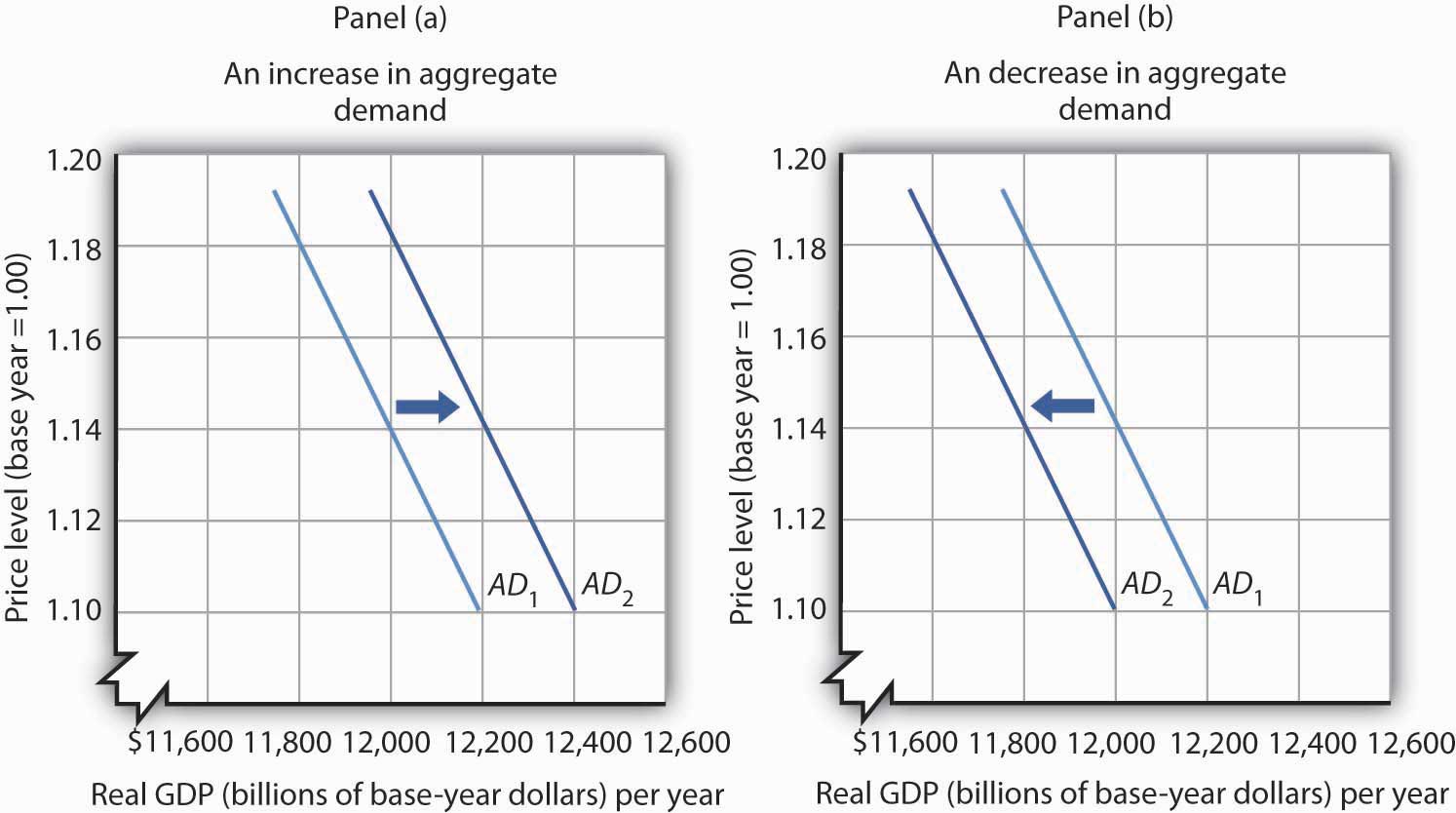
An increase in consumption, investment, government purchases, or net exports shifts the aggregate demand curve AD1 to the right as shown in Panel (a). A reduction in one of the components of aggregate demand shifts the curve to the left, as shown in Panel (b).
What factors might cause the aggregate demand curve to shift? Each of the components of aggregate demand is a possible aggregate demand shifter. We shall look at some of the events that can trigger changes in the components of aggregate demand and thus shift the aggregate demand curve.
Changes in Consumption
Several events could change the quantity of consumption at each price level and thus shift aggregate demand. One determinant of consumption is consumer confidence. If consumers expect good economic conditions and are optimistic about their economic prospects, they are more likely to buy major items such as cars or furniture. The result would be an increase in the real value of consumption at each price level and an increase in aggregate demand. In the second half of the 1990s, sustained economic growth and low unemployment fueled high expectations and consumer optimism. Surveys revealed consumer confidence to be very high. That consumer confidence translated into increased consumption and increased aggregate demand. In contrast, a decrease in consumption would accompany diminished consumer expectations and a decrease in consumer confidence, as happened after the stock market crash of 1929. The same problem has plagued the economies of most Western nations in 2008 as declining consumer confidence has tended to reduce consumption. A survey by the Conference Board in September of 2008 showed that just 13.5% of consumers surveyed expected economic conditions in the United States to improve in the next six months. Similarly pessimistic views prevailed in the previous two months. That contributed to the decline in consumption that occurred in the third quarter of the year.
Another factor that can change consumption and shift aggregate demand is tax policy. A cut in personal income taxes leaves people with more after-tax income, which may induce them to increase their consumption. The federal government in the United States cut taxes in 1964, 1981, 1986, 1997, and 2003; each of those tax cuts tended to increase consumption and aggregate demand at each price level.
In the United States, another government policy aimed at increasing consumption and thus aggregate demand has been the use of rebates in which taxpayers are simply sent checks in hopes that those checks will be used for consumption. Rebates have been used in 1975, 2001, and 2008. In each case the rebate was a one-time payment. Careful studies by economists of the 1975 and 2001 rebates showed little impact on consumption. Final evidence on the impact of the 2008 rebates is not yet in, but early results suggest a similar outcome. In a subsequent chapter, we will investigate arguments about whether temporary increases in income produced by rebates are likely to have a significant impact on consumption.
Transfer payments such as welfare and Social Security also affect the income people have available to spend. At any given price level, an increase in transfer payments raises consumption and aggregate demand, and a reduction lowers consumption and aggregate demand.
Changes in Investment
Investment is the production of new capital that will be used for future production of goods and services. Firms make investment choices based on what they think they will be producing in the future. The expectations of firms thus play a critical role in determining investment. If firms expect their sales to go up, they are likely to increase their investment so that they can increase production and meet consumer demand. Such an increase in investment raises the aggregate quantity of goods and services demanded at each price level; it increases aggregate demand.
Changes in interest rates also affect investment and thus affect aggregate demand. We must be careful to distinguish such changes from the interest rate effect, which causes a movement along the aggregate demand curve. A change in interest rates that results from a change in the price level affects investment in a way that is already captured in the downward slope of the aggregate demand curve; it causes a movement along the curve. A change in interest rates for some other reason shifts the curve. We examine reasons interest rates might change in another chapter.
Investment can also be affected by tax policy. One provision of the Job and Growth Tax Relief Reconciliation Act of 2003 was a reduction in the tax rate on certain capital gains. Capital gains result when the owner of an asset, such as a house or a factory, sells the asset for more than its purchase price (less any depreciation claimed in earlier years). The lower capital gains tax could stimulate investment, because the owners of such assets know that they will lose less to taxes when they sell those assets, thus making assets subject to the tax more attractive.
Changes in Government Purchases
Any change in government purchases, all other things unchanged, will affect aggregate demand. An increase in government purchases increases aggregate demand; a decrease in government purchases decreases aggregate demand.
Many economists argued that reductions in defense spending in the wake of the collapse of the Soviet Union in 1991 tended to reduce aggregate demand. Similarly, increased defense spending for the wars in Afghanistan and Iraq increased aggregate demand. Dramatic increases in defense spending to fight World War II accounted in large part for the rapid recovery from the Great Depression.
Changes in Net Exports
A change in the value of net exports at each price level shifts the aggregate demand curve. A major determinant of net exports is foreign demand for a country’s goods and services; that demand will vary with foreign incomes. An increase in foreign incomes increases a country’s net exports and aggregate demand; a slump in foreign incomes reduces net exports and aggregate demand. For example, several major U.S. trading partners in Asia suffered recessions in 1997 and 1998. Lower real incomes in those countries reduced U.S. exports and tended to reduce aggregate demand.
Exchange rates also influence net exports, all other things unchanged. A country’s exchange rate is the price of its currency in terms of another currency or currencies. A rise in the U.S. exchange rate means that it takes more Japanese yen, for example, to purchase one dollar. That also means that U.S. traders get more yen per dollar. Since prices of goods produced in Japan are given in yen and prices of goods produced in the United States are given in dollars, a rise in the U.S. exchange rate increases the price to foreigners for goods and services produced in the United States, thus reducing U.S. exports; it reduces the price of foreign-produced goods and services for U.S. consumers, thus increasing imports to the United States. A higher exchange rate tends to reduce net exports, reducing aggregate demand. A lower exchange rate tends to increase net exports, increasing aggregate demand.
Foreign price levels can affect aggregate demand in the same way as exchange rates. For example, when foreign price levels fall relative to the price level in the United States, U.S. goods and services become relatively more expensive, reducing exports and boosting imports in the United States. Such a reduction in net exports reduces aggregate demand. An increase in foreign prices relative to U.S. prices has the opposite effect.
The trade policies of various countries can also affect net exports. A policy by Japan to increase its imports of goods and services from India, for example, would increase net exports in India.
The Multiplier
A change in any component of aggregate demand shifts the aggregate demand curve. Generally, the aggregate demand curve shifts by more than the amount by which the component initially causing it to shift changes.
Suppose that net exports increase due to an increase in foreign incomes. As foreign demand for domestically made products rises, a country’s firms will hire additional workers or perhaps increase the average number of hours that their employees work. In either case, incomes will rise, and higher incomes will lead to an increase in consumption. Taking into account these other increases in the components of aggregate demand, the aggregate demand curve will shift by more than the initial shift caused by the initial increase in net exports.
The multiplierThe ratio of the change in the quantity of real GDP demanded at each price level to the initial change in one or more components of aggregate demand that produced it. is the ratio of the change in the quantity of real GDP demanded at each price level to the initial change in one or more components of aggregate demand that produced it:
Equation 22.1
[latex]Multiplier = \frac{ \Delta (real \: GDP \: demanded \: at \: each \: price \: level)}{ initial \Delta (component \: of \: AD)}[/latex]
We use the capital Greek letter delta (Δ) to mean “change in.” In the aggregate demand–aggregate supply model presented in this chapter, it is the number by which we multiply an initial change in aggregate demand to obtain the amount by which the aggregate demand curve shifts as a result of the initial change. In other words, we can use Equation 22.1 to solve for the change in real GDP demanded at each price level:
Equation 22.2
[latex]\Delta (real \: GDP \: demanded \: at \: each \: price \: level) = multiplier \times initial \: \Delta (component \: of \: AD)[/latex]
Suppose that the initial increase in net exports is $100 billion and that the initial $100-billion increase generates additional consumption of $100 billion at each price level. In Panel (a) of Figure 22.3 “The Multiplier”, the aggregate demand curve shifts to the right by $200 billion—the amount of the initial increase in net exports times the multiplier of 2. We obtained the value for the multiplier in this example by plugging $200 billion (the initial $100-billion increase in net exports plus the $100-billion increase that it generated in consumption) into the numerator of Equation 22.1 and $100 billion into the denominator. Similarly, a decrease in net exports of $100 billion leads to a decrease in aggregate demand of $200 billion at each price level, as shown in Panel (b).
Figure 22.3 The Multiplier
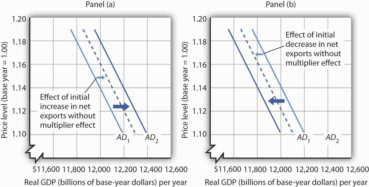
A change in one component of aggregate demand shifts the aggregate demand curve by more than the initial change. In Panel (a), an initial increase of $100 billion of net exports shifts the aggregate demand curve to the right by $200 billion at each price level. In Panel (b), a decrease of net exports of $100 billion shifts the aggregate demand curve to the left by $200 billion. In this example, the multiplier is 2.
Key Takeaways
- Potential output is the level of output an economy can achieve when labor is employed at its natural level. When an economy fails to produce at its potential, the government or the central bank may try to push the economy toward its potential.
- The aggregate demand curve represents the total of consumption, investment, government purchases, and net exports at each price level in any period. It slopes downward because of the wealth effect on consumption, the interest rate effect on investment, and the international trade effect on net exports.
- The aggregate demand curve shifts when the quantity of real GDP demanded at each price level changes.
- The multiplier is the number by which we multiply an initial change in aggregate demand to obtain the amount by which the aggregate demand curve shifts at each price level as a result of the initial change.
Try It!
Explain the effect of each of the following on the aggregate demand curve for the United States:
- A decrease in consumer optimism
- An increase in real GDP in the countries that buy U.S. exports
- An increase in the price level
- An increase in government spending on highways
Case in Point: The Multiplied Economic Impact of SARS on China’s Economy
Figure 22.4

Zervas – wrong face mask – CC BY-NC-ND 2.0.
Severe Acute Respiratory Syndrome (SARS), an atypical pneumonia-like disease, broke onto the world scene in late 2002. In March 2003, the World Health Organization (WHO) issued its first worldwide alert and a month later its first travel advisory, which recommended that travelers avoid Hong Kong and the southern province of China, Guangdong. Over the next few months, additional travel advisories were issued for other parts of China, Taiwan, and briefly for Toronto, Canada. By the end of June, all WHO travel advisories had been removed.
To estimate the overall impact of SARS on the Chinese economy in 2003, economists Wen Hai, Zhong Zhao, and Jian Want of Peking University’s China Center for Economic Research conducted a survey of Beijing’s tourism industry in April 2003. Based on findings from the Beijing area, they projected the tourism sector of China as a whole would lose $16.8 billion—of which $10.8 billion came from an approximate 50% reduction in foreign tourist revenue and $6 billion from curtailed domestic tourism, as holiday celebrations were cancelled and domestic travel restrictions imposed.
To figure out the total impact of SARS on China’s economy, they argued that the multiplier for tourism revenue in China is between 2 and 3. Since the SARS outbreak only began to have a major economic impact after March, they assumed a smaller multiplier of 1.5 for all of 2003. They thus predicted that the Chinese economy would be $25.3 billion smaller in 2003 as a result of SARS:
Source: Wen Hai, Zhong Zhao, and Jian Wan, “The Short-Term Impact of SARS on the Chinese Economy,” Asian Economic Papers 3, no. 1 (Winter 2004): 57–61.
Answer to Try It! Problem
- A decline in consumer optimism would cause the aggregate demand curve to shift to the left. If consumers are more pessimistic about the future, they are likely to cut purchases, especially of major items.
- An increase in the real GDP of other countries would increase the demand for U.S. exports and cause the aggregate demand curve to shift to the right. Higher incomes in other countries will make consumers in those countries more willing and able to buy U.S. goods.
- An increase in the price level corresponds to a movement up along the unchanged aggregate demand curve. At the higher price level, the consumption, investment, and net export components of aggregate demand will all fall; that is, there will be a reduction in the total quantity of goods and services demanded, but not a shift of the aggregate demand curve itself.
- An increase in government spending on highways means an increase in government purchases. The aggregate demand curve would shift to the right.
