4.2 Government Intervention in Market Prices: Price Floors and Price Ceilings
Learning Objectives
- Use the model of demand and supply to explain what happens when the government imposes price floors or price ceilings.
- Discuss the reasons why governments sometimes choose to control prices and the consequences of price control policies.
So far in this chapter and in the previous chapter, we have learned that markets tend to move toward their equilibrium prices and quantities. Surpluses and shortages of goods are short-lived as prices adjust to equate quantity demanded with quantity supplied.
In some markets, however, governments have been called on by groups of citizens to intervene to keep prices of certain items higher or lower than what would result from the market finding its own equilibrium price. In this section we will examine agricultural markets and apartment rental markets—two markets that have often been subject to price controls. Through these examples, we will identify the effects of controlling prices. In each case, we will look at reasons why governments have chosen to control prices in these markets and the consequences of these policies.
Agricultural Price Floors
Governments often seek to assist farmers by setting price floors in agricultural markets. A minimum allowable price set above the equilibrium price is a price floor. With a price floor, the government forbids a price below the minimum. (Notice that, if the price floor were for whatever reason set below the equilibrium price, it would be irrelevant to the determination of the price in the market since nothing would prohibit the price from rising to equilibrium.) A price floor that is set above the equilibrium price creates a surplus.
Figure 4.8 “Price Floors in Wheat Markets” shows the market for wheat. Suppose the government sets the price of wheat at PF. Notice that PF is above the equilibrium price of PE. At PF, we read over to the demand curve to find that the quantity of wheat that buyers will be willing and able to purchase is W1 bushels. Reading over to the supply curve, we find that sellers will offer W2 bushels of wheat at the price floor of PF. Because PF is above the equilibrium price, there is a surplus of wheat equal to (W2 − W1) bushels. The surplus persists because the government does not allow the price to fall.
Figure 4.8 Price Floors in Wheat Markets
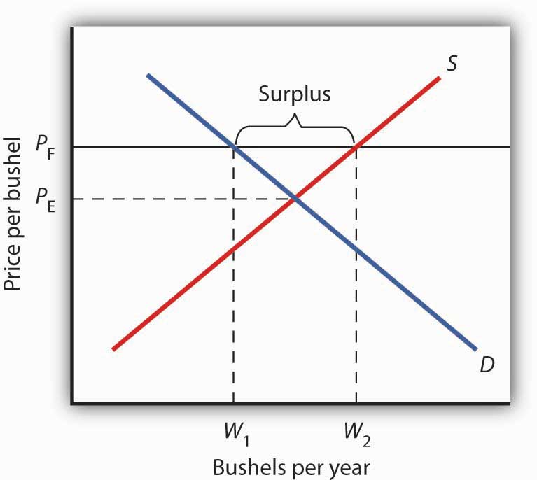
A price floor for wheat creates a surplus of wheat equal to (W2 – W1) bushels.
Why have many governments around the world set price floors in agricultural markets? Farming has changed dramatically over the past two centuries. Technological improvements in the form of new equipment, fertilizers, pesticides, and new varieties of crops have led to dramatic increases in crop output per acre. Worldwide production capacity has expanded markedly. As we have learned, technological improvements cause the supply curve to shift to the right, reducing the price of food. While such price reductions have been celebrated in computer markets, farmers have successfully lobbied for government programs aimed at keeping their prices from falling.
While the supply curve for agricultural goods has shifted to the right, the demand has increased with rising population and with rising income. But as incomes rise, people spend a smaller and smaller fraction of their incomes on food. While the demand for food has increased, that increase has not been nearly as great as the increase in supply. Figure 4.9 “Supply and Demand Shifts for Agricultural Products” shows that the supply curve has shifted much farther to the right, from S1 to S2, than the demand curve has, from D1 to D2. As a result, equilibrium quantity has risen dramatically, from Q1 to Q2, and equilibrium price has fallen, from P1 to P2.
On top of this long-term historical trend in agriculture, agricultural prices are subject to wide swings over shorter periods. Droughts or freezes can sharply reduce supplies of particular crops, causing sudden increases in prices. Demand for agricultural goods of one country can suddenly dry up if the government of another country imposes trade restrictions against its products, and prices can fall. Such dramatic shifts in prices and quantities make incomes of farmers unstable.
Figure 4.9 Supply and Demand Shifts for Agricultural Products
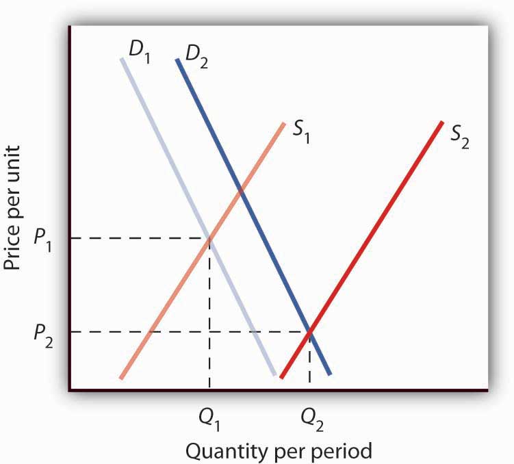
A relatively large increase in the supply of agricultural products, accompanied by a relatively small increase in demand, has reduced the price received by farmers and increased the quantity of agricultural goods.
The Great Depression of the 1930s led to a major federal role in agriculture. The Depression affected the entire economy, but it hit farmers particularly hard. Prices received by farmers plunged nearly two-thirds from 1930 to 1933. Many farmers had a tough time keeping up mortgage payments. By 1932, more than half of all farm loans were in default.
Farm legislation passed during the Great Depression has been modified many times, but the federal government has continued its direct involvement in agricultural markets. This has meant a variety of government programs that guarantee a minimum price for some types of agricultural products. These programs have been accompanied by government purchases of any surplus, by requirements to restrict acreage in order to limit those surpluses, by crop or production restrictions, and the like.
To see how such policies work, look back at Figure 4.8 “Price Floors in Wheat Markets”. At PF, W2 bushels of wheat will be supplied. With that much wheat on the market, there is market pressure on the price of wheat to fall. To prevent price from falling, the government buys the surplus of (W2 – W1) bushels of wheat, so that only W1 bushels are actually available to private consumers for purchase on the market. The government can store the surpluses or find special uses for them. For example, surpluses generated in the United States have been shipped to developing countries as grants-in-aid or distributed to local school lunch programs. As a variation on this program, the government can require farmers who want to participate in the price support program to reduce acreage in order to limit the size of the surpluses.
After 1973, the government stopped buying the surpluses (with some exceptions) and simply guaranteed farmers a “target price.” If the average market price for a crop fell below the crop’s target price, the government paid the difference. If, for example, a crop had a market price of $3 per unit and a target price of $4 per unit, the government would give farmers a payment of $1 for each unit sold. Farmers would thus receive the market price of $3 plus a government payment of $1 per unit. For farmers to receive these payments, they had to agree to remove acres from production and to comply with certain conservation provisions. These restrictions sought to reduce the size of the surplus generated by the target price, which acted as a kind of price floor.
What are the effects of such farm support programs? The intention is to boost and stabilize farm incomes. But, with price floors, consumers pay more for food than they would otherwise, and governments spend heavily to finance the programs. With the target price approach, consumers pay less, but government financing of the program continues. U.S. federal spending for agriculture averaged well over $22 billion per year between 2003 and 2007, roughly $70 per person.
Help to farmers has sometimes been justified on the grounds that it boosts incomes of “small” farmers. However, since farm aid has generally been allotted on the basis of how much farms produce rather than on a per-farm basis, most federal farm support has gone to the largest farms. If the goal is to eliminate poverty among farmers, farm aid could be redesigned to supplement the incomes of small or poor farmers rather than to undermine the functioning of agricultural markets.
In 1996, the U.S. Congress passed the Federal Agriculture Improvement and Reform Act of 1996, or FAIR. The thrust of the new legislation was to do away with the various programs of price support for most crops and hence provide incentives for farmers to respond to market price signals. To protect farmers through a transition period, the act provided for continued payments that were scheduled to decline over a seven-year period. However, with prices for many crops falling in 1998, the U.S. Congress passed an emergency aid package that increased payments to farmers. In 2008, as farm prices reached record highs, Congress passed a farm bill that increased subsidy payments to $40 billion. It did, however, for the first time limit payments to the wealthiest farmers. Individual farmers whose farm incomes exceed $750,000 (or $1.5 million for couples) would be ineligible for some subsidy programs.
Rental Price Ceilings
The purpose of rent control is to make rental units cheaper for tenants than they would otherwise be. Unlike agricultural price controls, rent control in the United States has been largely a local phenomenon, although there were national rent controls in effect during World War II. Currently, about 200 cities and counties have some type of rent control provisions, and about 10% of rental units in the United States are now subject to price controls. New York City’s rent control program, which began in 1943, is among the oldest in the country. Many other cities in the United States adopted some form of rent control in the 1970s. Rent controls have been pervasive in Europe since World War I, and many large cities in poorer countries have also adopted rent controls.
Rent controls in different cities differ in terms of their flexibility. Some cities allow rent increases for specified reasons, such as to make improvements in apartments or to allow rents to keep pace with price increases elsewhere in the economy. Often, rental housing constructed after the imposition of the rent control ordinances is exempted. Apartments that are vacated may also be decontrolled. For simplicity, the model presented here assumes that apartment rents are controlled at a price that does not change.
Figure 4.10 Effect of a Price Ceiling on the Market for Apartments
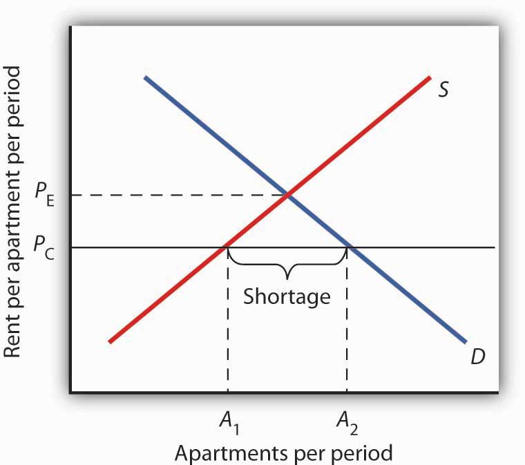
A price ceiling on apartment rents that is set below the equilibrium rent creates a shortage of apartments equal to (A2 − A1) apartments.
Figure 4.10 “Effect of a Price Ceiling on the Market for Apartments” shows the market for rental apartments. Notice that the demand and supply curves are drawn to look like all the other demand and supply curves you have encountered so far in this text: the demand curve is downward-sloping and the supply curve is upward-sloping.
The demand curve shows that a higher price (rent) reduces the quantity of apartments demanded. For example, with higher rents, more young people will choose to live at home with their parents. With lower rents, more will choose to live in apartments. Higher rents may encourage more apartment sharing; lower rents would induce more people to live alone.
The supply curve is drawn to show that as rent increases, property owners will be encouraged to offer more apartments to rent. Even though an aerial photograph of a city would show apartments to be fixed at a point in time, owners of those properties will decide how many to rent depending on the amount of rent they anticipate. Higher rents may also induce some homeowners to rent out apartment space. In addition, renting out apartments implies a certain level of service to renters, so that low rents may lead some property owners to keep some apartments vacant.
Rent control is an example of a price ceiling, a maximum allowable price. With a price ceiling, the government forbids a price above the maximum. A price ceiling that is set below the equilibrium price creates a shortage that will persist.
Suppose the government sets the price of an apartment at PC in Figure 4.10 “Effect of a Price Ceiling on the Market for Apartments”. Notice that PC is below the equilibrium price of PE. At PC, we read over to the supply curve to find that sellers are willing to offer A1 apartments. Reading over to the demand curve, we find that consumers would like to rent A2 apartments at the price ceiling of PC. Because PC is below the equilibrium price, there is a shortage of apartments equal to (A2 – A1). (Notice that if the price ceiling were set above the equilibrium price it would have no effect on the market since the law would not prohibit the price from settling at an equilibrium price that is lower than the price ceiling.)
Figure 4.11 The Unintended Consequences of Rent Control
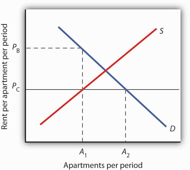
Controlling apartment rents at PC creates a shortage of (A2 − A1) apartments. For A1 apartments, consumers are willing and able to pay PB, which leads to various “backdoor” payments to apartment owners.
If rent control creates a shortage of apartments, why do some citizens nonetheless clamor for rent control and why do governments often give in to the demands? The reason generally given for rent control is to keep apartments affordable for low- and middle-income tenants.
But the reduced quantity of apartments supplied must be rationed in some way, since, at the price ceiling, the quantity demanded would exceed the quantity supplied. Current occupants may be reluctant to leave their dwellings because finding other apartments will be difficult. As apartments do become available, there will be a line of potential renters waiting to fill them, any of whom is willing to pay the controlled price of PC or more. In fact, reading up to the demand curve in Figure 4.11 “The Unintended Consequences of Rent Control” from A1 apartments, the quantity available at PC, you can see that for A1 apartments, there are potential renters willing and able to pay PB. This often leads to various “backdoor” payments to apartment owners, such as large security deposits, payments for things renters may not want (such as furniture), so-called “key” payments (“The monthly rent is $500 and the key price is $3,000”), or simple bribes.
In the end, rent controls and other price ceilings often end up hurting some of the people they are intended to help. Many people will have trouble finding apartments to rent. Ironically, some of those who do find apartments may actually end up paying more than they would have paid in the absence of rent control. And many of the people that the rent controls do help (primarily current occupants, regardless of their income, and those lucky enough to find apartments) are not those they are intended to help (the poor). There are also costs in government administration and enforcement.
Because New York City has the longest history of rent controls of any city in the United States, its program has been widely studied. There is general agreement that the rent control program has reduced tenant mobility, led to a substantial gap between rents on controlled and uncontrolled units, and favored long-term residents at the expense of newcomers to the city (Arnott, R., 1995). These distortions have grown over time, another frequent consequence of price controls.
A more direct means of helping poor tenants, one that would avoid interfering with the functioning of the market, would be to subsidize their incomes. As with price floors, interfering with the market mechanism may solve one problem, but it creates many others at the same time.
Key Takeaways
- Price floors create surpluses by fixing the price above the equilibrium price. At the price set by the floor, the quantity supplied exceeds the quantity demanded.
- In agriculture, price floors have created persistent surpluses of a wide range of agricultural commodities. Governments typically purchase the amount of the surplus or impose production restrictions in an attempt to reduce the surplus.
- Price ceilings create shortages by setting the price below the equilibrium. At the ceiling price, the quantity demanded exceeds the quantity supplied.
- Rent controls are an example of a price ceiling, and thus they create shortages of rental housing.
- It is sometimes the case that rent controls create “backdoor” arrangements, ranging from requirements that tenants rent items that they do not want to outright bribes, that result in rents higher than would exist in the absence of the ceiling.
Try It!
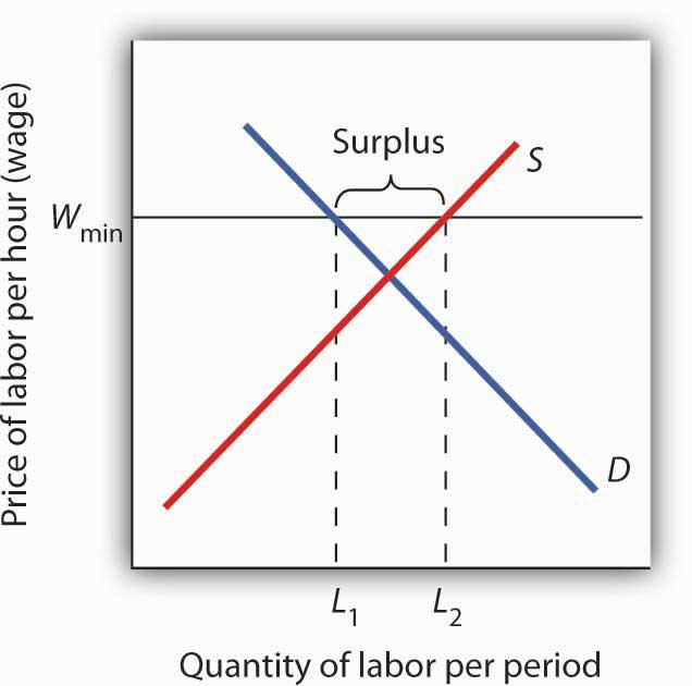
A minimum wage law is another example of a price floor. Draw demand and supply curves for unskilled labor. The horizontal axis will show the quantity of unskilled labor per period and the vertical axis will show the hourly wage rate for unskilled workers, which is the price of unskilled labor. Show and explain the effect of a minimum wage that is above the equilibrium wage.
Case in Point: Corn: It Is Not Just Food Any More

Government support for corn dates back to the Agricultural Act of 1938 and, in one form or another, has been part of agricultural legislation ever since. Types of supports have ranged from government purchases of surpluses to target pricing, land set asides, and loan guarantees. According to one estimate, the U.S. government spent nearly $42 billion to support corn between 1995 and 2004.
Then, during the period of rising oil prices of the late 1970s and mounting concerns about dependence on foreign oil from volatile regions in the world, support for corn, not as a food, but rather as an input into the production of ethanol—an alternative to oil-based fuel—began. Ethanol tax credits were part of the Energy Act of 1978. Since 1980, a tariff of 50¢ per gallon against imported ethanol, even higher today, has served to protect domestic corn-based ethanol from imported ethanol, in particular from sugar-cane-based ethanol from Brazil.
The Energy Policy Act of 2005 was another milestone in ethanol legislation. Through loan guarantees, support for research and development, and tax credits, it mandated that 4 billion gallons of ethanol be used by 2006 and 7.5 billion gallons by 2012. Ethanol production had already reached 6.5 billion gallons by 2007, so new legislation in 2007 upped the ante to 15 billion gallons by 2015.
Beyond the increased amount the government is spending to support corn and corn-based ethanol, criticism of the policy has three major prongs:
- Corn-based ethanol does little to reduce U.S. dependence on foreign oil because the energy required to produce a gallon of corn-based ethanol is quite high. A 2006 National Academy of Sciences paper estimated that one gallon of ethanol is needed to bring 1.25 gallons of it to market. Other studies show an even less favorable ratio.
- Biofuels, such as corn-based ethanol, are having detrimental effects on the environment, with increased deforestation, stemming from more land being used to grow fuel inputs, contributing to global warming.
- The diversion of corn and other crops from food to fuel is contributing to rising food prices and an increase in world hunger. C. Ford Runge and Benjamin Senauer wrote in Foreign Affairs that even small increases in prices of food staples have severe consequences on the very poor of the world, and “Filling the 25-gallon tank of an SUV with pure ethanol requires over 450 pounds of corn—which contains enough calories to feed one person for a year.”
Some of these criticisms may be contested as exaggerated: Will the ratio of energy-in to energy-out improve as new technologies emerge for producing ethanol? Did not other factors, such as weather and rising food demand worldwide, contribute to higher grain prices? Nonetheless, it is clear that corn-based ethanol is no free lunch. It is also clear that the end of government support for corn is nowhere to be seen.
Sources: Alexei Barrionuevo, “Mountains of Corn and a Sea of Farm Subsidies,” New York Times, November 9, 2005, online version; David Freddoso, “Children of the Corn,” National Review Online, May 6, 2008; C. Ford Runge and Benjamin Senauer, “How Biofuels Could Starve the Poor,” Foreign Affairs, May/June 2007, online version; Michael Grunwald, “The Clean Energy Scam,” Time 171:14 (April 7, 2008): 40–45.
Answer to Try It! Problem
A minimum wage (Wmin) that is set above the equilibrium wage would create a surplus of unskilled labor equal to (L2 – L1). That is, L2 units of unskilled labor are offered at the minimum wage, but companies only want to use L1 units at that wage. Because unskilled workers are a substitute for a skilled workers, forcing the price of unskilled workers higher would increase the demand for skilled labor and thus increase their wages.
Figure 4.13
References
Arnott, R., “Time for Revisionism on Rent Control,” Journal of Economic Perspectives 9(1) (Winter, 1995): 99–120.
