31.3 Inflation and Unemployment in the Long Run
Learning Objectives
- Use the equation of exchange to explain what determines the inflation rate in the long run.
- Explain why in the long run the Phillips curve is vertical.
- Describe frictional and structural unemployment and the factors that may affect these two types of unemployment.
- Describe efficiency wage theory and its predictions concerning cyclical unemployment.
In the last section, we saw how stabilization policy, together with changes in expectations, can produce the cycles of inflation and unemployment that characterized the past several decades. These cycles, though, are short-run phenomena. They involve swings in economic activity around the economy’s potential output.
This section examines forces that affect the values of inflation and the unemployment rate in the long run. We shall see that the rates of money growth and of economic growth determine the inflation rate. Unemployment that persists in the long run includes frictional and structural unemployment. We shall examine some of the forces that affect both types of unemployment, as well as a new theory of unemployment.
The Inflation Rate in the Long Run
What factors determine the inflation rate? The price level is determined by the intersection of aggregate demand and short-run aggregate supply; anything that shifts either of these two curves changes the price level and thus affects the inflation rate. We have seen how these shifts can generate different inflation–unemployment combinations in the short run. In the long run, the rate of inflation will be determined by two factors: the rate of money growth and the rate of economic growth.
Economists generally agree that the rate of money growth is one determinant of an economy’s inflation rate in the long run. The conceptual basis for that conclusion lies in the equation of exchange: MV = PY. That is, the money supply times the velocity of money equals the price level times the value of real GDP.
Given the equation of exchange, which holds by definition, we learned in the chapter on monetary policy that the sum of the percentage rates of change in M and V will be roughly equal to the sum of the percentage rates of change in P and Y. That is,
Equation 31.1
[latex]\% \Delta M + \% \Delta V \cong \% \Delta P + \% \Delta Y[/latex]
Suppose that velocity is stable in the long run, so that %ΔV equals zero. Then, the inflation rate (%ΔP) roughly equals the percentage rate of change in the money supply minus the percentage rate of change in real GDP:
Equation 31.2
[latex]\% \Delta P \cong \% \Delta M \: - \: \% \Delta Y[/latex]
In the long run, real GDP moves to its potential level, YP. Thus, in the long run we can write Equation 31.2 as follows:
Equation 31.3
[latex]\% \Delta P \cong \% \Delta M \: - \: \% \Delta Y_P[/latex]
There is a limit to how fast the economy’s potential output can grow. Economists generally agree that potential output increases at only about a 2% to 3% annual rate in the United States. Given that the economy stays close to its potential, this puts a rough limit on the speed with which Y can grow. Velocity can vary, but it is not likely to change at a rapid rate over a sustained period. These two facts suggest that very rapid increases in the quantity of money, M, will inevitably produce very rapid increases in the price level, P. If the money supply grows more slowly than potential output, then the right-hand side of Equation 31.3 will be negative. The price level will fall; the economy experiences deflation.
Numerous studies point to the strong relationship between money growth and inflation, especially for high-inflation countries. Figure 31.13 “Money Growth Rates and Inflation over the Long Run” is from a recent study by economists Paul De Grauwe and Magdalena Polan. It is based on a sample of 160 countries over a 30-year period. Panel (a) includes all 160 countries and suggests a positive relationship between money growth and the rate of inflation. The relationship is clearly not precise, and the relationship is strengthened by the presence of countries with very high inflation rates. When the researchers break down the sample into countries with inflation rates of less than 10%, less than 20%, and less than 50%, they find that for countries with single-digit inflation the relationship between inflation and money growth is quite weak. Panel (b) shows that there is still a visible, though of course not perfect, correlation when examining countries with inflation rates of less than 50% (Grauwe & Polan, 2005).
Figure 31.13 Money Growth Rates and Inflation over the Long Run
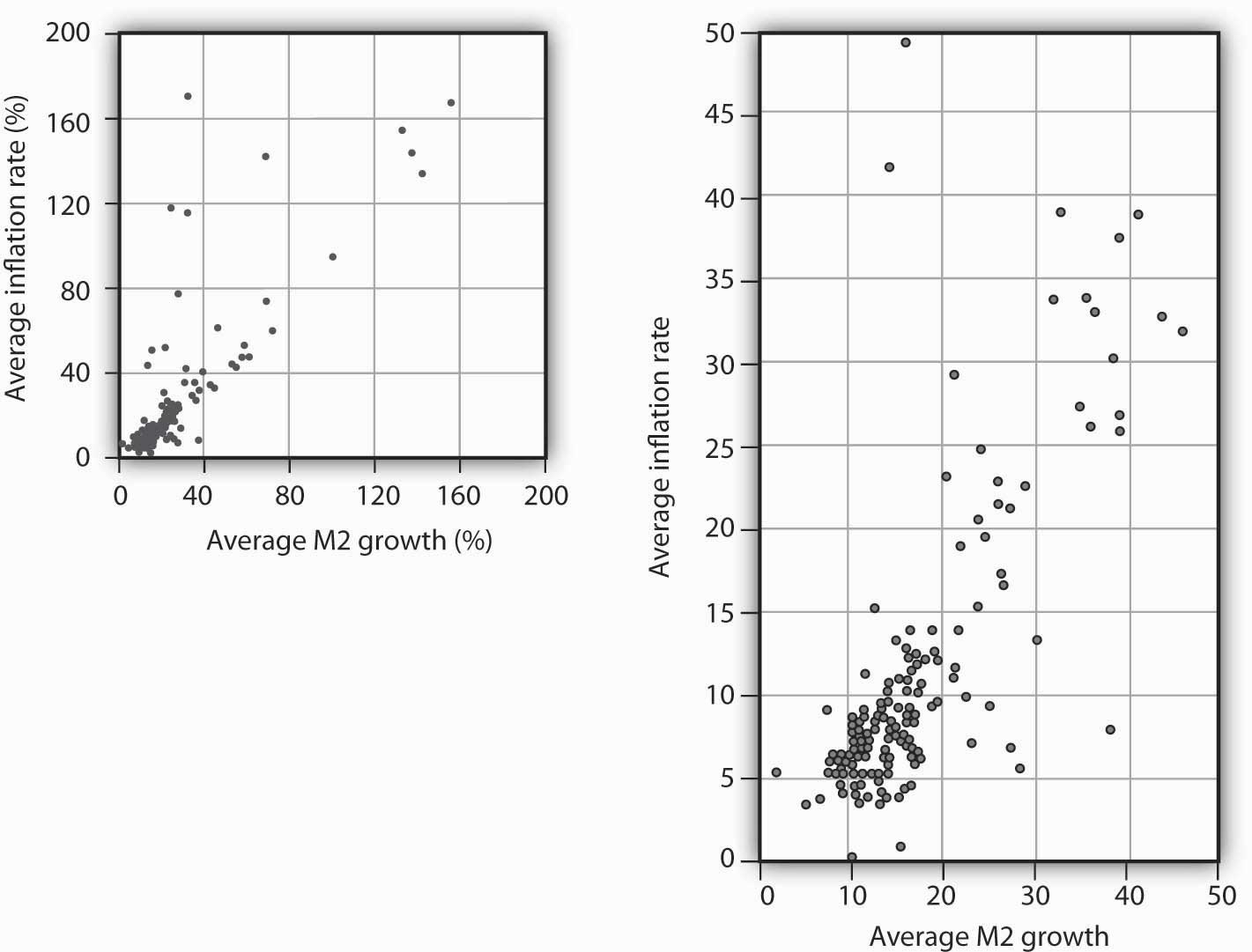
Data for 160 countries over a 30-year period suggest a positive relationship between the rate of money growth and inflation. The graph shows the inflation rate against a broad definition of the money supply, M2.
Source: Paul De Grauwe and Magdalena Polan, “Is Inflation Always and Everywhere a Monetary Phenomenon?” Scandinavian Journal of Economics 107, no. 2 (2005): 245–46.
In the model of aggregate demand and aggregate supply, increases in the money supply shift the aggregate demand curve to the right and thus force the price level upward. Money growth thus produces inflation.
Of course, other factors can shift the aggregate demand curve as well. For example, expansionary fiscal policy or an increase in investment will shift aggregate demand. We have already seen that changes in the expected price level or in production costs shift the short-run aggregate supply curve. But such increases are not likely to continue year after year, as money growth can. Factors other than money growth may influence the inflation rate from one year to the next, but they are not likely to cause sustained inflation.
Inflation Rates and Economic Growth
Our conclusion is a simple and an important one. In the long run, the inflation rate is determined by the relative values of the economy’s rate of money growth and of its rate of economic growth. If the money supply increases more rapidly than the rate of economic growth, inflation is likely to result. A money growth rate equal to the rate of economic growth will, in the absence of a change in velocity, produce a zero rate of inflation. Finally, a money growth rate that falls short of the rate of economic growth is likely to lead to deflation.
Unemployment in the Long Run
Economists distinguish three types of unemployment: frictional unemployment, structural unemployment, and cyclical unemployment. The first two exist at all times, even when the economy operates at its potential. These two types of unemployment together determine the natural rate of unemployment. In the long run, the economy will operate at potential, and the unemployment rate will be the natural rate of unemployment. For this reason, in the long run the Phillips curve will be vertical at the natural rate of unemployment. Figure 31.14 “The Phillips Curve in the Long Run” explains why. Suppose the economy is operating at YP on AD1 and SRAS1. Suppose the price level is P0, the same as in the last period. In that case, the inflation rate is 0. Panel (b) shows that the unemployment rate is UP, the natural rate of unemployment. Now suppose that the aggregate demand curve shifts to AD2. In the short run, output will increase to Y1. The price level will rise to P1, and the unemployment rate will fall to U1. In Panel (b) we show the new unemployment rate, U1, to be associated with an inflation rate of π1, and the beginnings of the negatively sloped short-run Phillips curve emerges. In the long run, as price and nominal wages increase, the short-run aggregate supply curve moves to SRAS2 and output returns to YP, as shown in Panel (a). In Panel (b), unemployment returns to UP, regardless of the rate of inflation. Thus, in the long-run, the Phillips curve is vertical.
Figure 31.14 The Phillips Curve in the Long Run
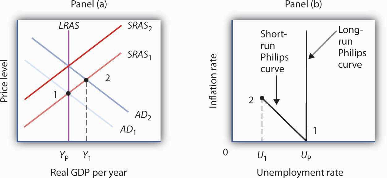
Suppose the economy is operating at YP on AD1 and SRAS1 in Panel (a) with price level of P0, the same as in the last period. Panel (b) shows that the unemployment rate is UP, the natural rate of unemployment. If the aggregate demand curve shifts to AD2, in the short run output will increase to Y1, and the price level will rise to P1. In Panel (b), the unemployment rate will fall to U1, and the inflation rate will be π1. In the long run, as price and nominal wages increase, the short-run aggregate supply curve moves to SRAS2, and output returns to YP, as shown in Panel (a). In Panel (b), unemployment returns to UP, regardless of the rate of inflation. Thus, in the long-run, the Phillips curve is vertical.
An economy operating at its potential would have no cyclical unemployment. Because an economy achieves its potential output in the long run, an analysis of unemployment in the long run is an analysis of frictional and structural unemployment. In this section, we will also look at some new research that challenges the very concept of an economy achieving its potential output.
Frictional Unemployment
Frictional unemployment occurs because it takes time for people seeking jobs and employers seeking workers to find each other. If the amount of time could be reduced, frictional unemployment would fall. The economy’s natural rate of unemployment would drop, and its potential output would rise. This section presents a model of frictional unemployment and examines some issues in reducing the frictional unemployment rate.
A period of frictional unemployment ends with the individual getting a job. The process through which the job is obtained suggests some important clues to the nature of frictional unemployment.
By definition, a person who is unemployed is seeking work. At the outset of a job search, we presume that the individual has a particular wage in mind as he or she considers various job possibilities. The lowest wage that an unemployed worker would accept, if it were offered, is called the reservation wage. This is the wage an individual would accept; any offer below it would be rejected. Once a firm offers the reservation wage, the individual will take it and the job search will be terminated. Many people may hold out for more than just a wage—they may be seeking a certain set of working conditions, opportunities for advancement, or a job in a particular area. In practice, then, an unemployed worker might be willing to accept a variety of combinations of wages and other job characteristics. We shall simplify our analysis by lumping all these other characteristics into a single reservation wage.
A worker’s reservation wage is likely to change as his or her search continues. One might initiate a job search with high expectations and thus have a high reservation wage. As the job search continues, however, this reservation wage might be adjusted downward as the worker obtains better information about what is likely to be available in the market and as the financial difficulties associated with unemployment mount. We can thus draw a reservation wage curve (Figure 31.15 “A Model of a Job Search”), that suggests a negative relationship between the reservation wage and the duration of a person’s job search. Similarly, as a job search continues, the worker will accumulate better offers. The “best-offer-received” curve shows what its name implies; it is the best offer the individual has received so far in the job search. The upward slope of the curve suggests that, as a worker’s search continues, the best offer received will rise.
Figure 31.15 A Model of a Job Search

An individual begins a job search at time t0 with a reservation wage W0. As long as the reservation wage exceeds the best offer received, the individual will continue searching. A job is accepted, and the search is terminated, at time tc, at which the reservation and “best-offer-received” curves intersect at wage Wc.
The search begins at time t0, with the unemployed worker seeking wage W0. Because the worker’s reservation wage exceeds the best offer received, the worker continues the search. The worker reduces his or her reservation wage and accumulates better offers until the two curves intersect at time tc. The worker accepts wage Wc, and the job search is terminated.
The job search model in Figure 31.15 “A Model of a Job Search” does not determine an equilibrium duration of job search or an equilibrium initial wage. The reservation wage and best-offer-received curves will be unique to each individual’s experience. We can, however, use the model to reach some conclusions about factors that affect frictional unemployment.
First, the duration of search will be shorter when more job market information is available. Suppose, for example, that the only way to determine what jobs and wages are available is to visit each firm separately. Such a situation would require a lengthy period of search before a given offer was received. Alternatively, suppose there are agencies that make such information readily available and that link unemployed workers to firms seeking to hire workers. In that second situation, the time required to obtain a given offer would be reduced, and the best-offer-received curves for individual workers would shift to the left. The lower the cost for obtaining job market information, the lower the average duration of unemployment. Government and private agencies that provide job information and placement services help to reduce information costs to unemployed workers and firms. They tend to lower frictional unemployment by shifting the best-offer-received curves for individual workers to the left, as shown in Panel (a) of Figure 31.16 “Public Policy and Frictional Unemployment”. Workers obtain higher-paying jobs when they do find work; the wage at which searches are terminated rises to W2.
Figure 31.16 Public Policy and Frictional Unemployment
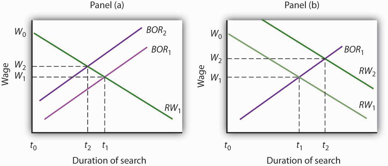
Public policy can influence the time required for job-seeking workers and worker-seeking firms to find each other. Programs that provide labor-market information tend to shift the best-offer-received (BOR) curves of individual workers to the left, reducing the duration of job search and reducing unemployment, as in Panel (a). Note that the wage these workers obtain also rises to W2. Unemployment compensation tends to increase the period over which a worker will hold out for a particular wage, shifting the reservation wage (RW) curve to the right, as in Panel (b). Unemployment compensation thus boosts the unemployment rate and increases the wage workers obtain when they find employment.
Unemployment compensation, which was introduced in the United States during the Great Depression to help workers who had lost jobs through unemployment, also affects frictional unemployment. Because unemployment compensation reduces the financial burden of being unemployed, it is likely to increase the amount of time people will wait for a given wage. It thus shifts the reservation wage curve to the right, raises the average duration of unemployment, and increases the wage at which searches end, as shown in Panel (b). An increase in the average duration of unemployment implies a higher unemployment rate. Unemployment compensation thus has a paradoxical effect—it tends to increase the problem against which it protects.
Structural Unemployment
Structural unemployment occurs when a firm is looking for a worker and an unemployed worker is looking for a job, but the particular characteristics the firm seeks do not match up with the characteristics the worker offers. Technological change is one source of structural unemployment. New technologies are likely to require different skills than old technologies. Workers with training to equip them for the old technology may find themselves caught up in a structural mismatch.
Technological and managerial changes have, for example, changed the characteristics firms seek in workers they hire. Firms looking for assembly-line workers once sought men and women with qualities such as reliability, integrity, strength, and manual dexterity. Reliability and integrity remain important, but many assembly-line jobs now require greater analytical and communications skills. Automobile manufacturers, for example, now test applicants for entry-level factory jobs on their abilities in algebra, in trigonometry, and in written and oral communications. Strong, agile workers with weak analytical and language skills may find many job openings for which they do not qualify. They would be examples of the structurally unemployed.
Changes in demand can also produce structural unemployment. As consumers shift their demands to different products, firms that are expanding and seeking more workers may need different skills than firms for which demand has shrunk. Similarly, firms may shift their use of different types of jobs in response to changing market conditions, leaving some workers with the “wrong” set of skills. Regional shifts in demand can produce structural unemployment as well. The economy of one region may be expanding rapidly, creating job vacancies, while another region is in a slump, with many workers seeking jobs but not finding them.
Public and private job training firms seek to reduce structural unemployment by providing workers with skills now in demand. Employment services that provide workers with information about jobs in other regions also reduce the extent of structural unemployment.
Cyclical Unemployment and Efficiency Wages
In our model, unemployment above the natural level occurs if, at a given real wage, the quantity of labor supplied exceeds the quantity of labor demanded. In the analysis we’ve done so far, the failure to achieve equilibrium is a short-run phenomenon. In the long run, wages and prices will adjust so that the real wage reaches its equilibrium level. Employment reaches its natural level.
Some economists, however, argue that a real wage that achieves equilibrium in the labor market may never be reached. They suggest that firms may intentionally pay a wage greater than the market equilibrium. Such firms could hire additional workers at a lower wage, but they choose not to do so. The idea that firms may hold to a real wage greater than the equilibrium wage is called efficiency-wage theory.
Why would a firm pay higher wages than the market requires? Suppose that by paying higher wages, the firm is able to boost the productivity of its workers. Workers become more contented and more eager to perform in ways that boost the firm’s profits. Workers who receive real wages above the equilibrium level may also be less likely to leave their jobs. That would reduce job turnover. A firm that pays its workers wages in excess of the equilibrium wage expects to gain by retaining its employees and by inducing those employees to be more productive. Efficiency-wage theory thus suggests that the labor market may divide into two segments. Workers with jobs will receive high wages. Workers without jobs, who would be willing to work at an even lower wage than the workers with jobs, find themselves closed out of the market.
Whether efficiency wages really exist remains a controversial issue, but the argument is an important one. If it is correct, then the wage rigidity that perpetuates a recessionary gap is transformed from a temporary phenomenon that will be overcome in the long run to a permanent feature of the market. The argument implies that the ordinary processes of self-correction will not eliminate a recessionary gap1.
Key Takeaways
- Two factors that can influence the rate of inflation in the long run are the rate of money growth and the rate of economic growth.
- In the long run, the Phillips curve will be vertical since when output is at potential, the unemployment rate will be the natural rate of unemployment, regardless of the rate of inflation.
- The rate of frictional unemployment is affected by information costs and by the existence of unemployment compensation.
- Policies to reduce structural unemployment include the provision of job training and information about labor-market conditions in other regions.
- Efficiency-wage theory predicts that profit-maximizing firms will maintain the wage level at a rate too high to achieve full employment in the labor market.
Try It!
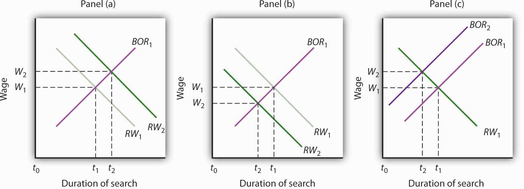
Using the model of a job search (see Figure 31.15 “A Model of a Job Search”), show graphically how each of the following would be likely to affect the duration of an unemployed worker’s job search and thus the unemployment rate:
- A new program provides that workers who have lost their jobs will receive unemployment compensation from the government equal to the pay they were earning when they lost their jobs, and that this compensation will continue for at least five years.
- Unemployment compensation is provided, but it falls by 20% each month a person is out of work.
- Access to the Internet becomes much more widely available and is used by firms looking for workers and by workers seeking jobs.
Case in Point: Altering the Incentives for Unemployment Insurance Claimants
Figure 31.17

Tax Credits – Unemployment – CC BY 2.0.
While the rationale for unemployment insurance is clear—to help people weather bouts of unemployment—especially during economic downturns, designing programs that reduce adverse incentives is challenging. A review article by economists Peter Fredriksson and Bertil Holmlund examined decades of research that looks at how unemployment insurance programs could be improved. In particular, they consider the value of changing the duration and profile of benefit payments, increasing monitoring and sanctions imposed on unemployment insurance recipients, and changing work requirements. Some of the research is theoretical, while some comes out of actual experiments.
Concerning benefit payments, they suggest that reducing payments over time provides better incentives than either keeping payments constant or increasing them over time. Research also suggests that a waiting period might also be useful. Concerning monitoring and sanctions, most unemployment insurance systems require claimants to demonstrate in some way that they have looked for work. For example, they must report regularly to employment agencies or provide evidence they have applied for jobs. If they do not, the benefit may be temporarily cut. A number of experiments support the notion that greater search requirements reduce the length of unemployment. One experiment conducted in Maryland assigned recipients to different processes ranging from the standard requirement at the time of two employer contacts per week to requiring at least four contacts per week, attending a four-day job search workshop, and telling claimants that their employer contacts would be verified. The results showed that increasing the number of employer contacts reduced the duration by 6%, attending the workshop reduced duration by 5%, and the possibility of verification reduced it by 7.5%. Indeed, just telling claimants that they were going to have to attend the workshop led to a reduction in claimants. Evidence on instituting some kind of work requirement is similar to that of instituting workshop attendance.
The authors conclude that the effectiveness of all these instruments results from the fact that they encourage more active job search.
Source: Peter Fredriksson and Bertil Holmlund, “Improving Incentives in Unemployment Insurance: A Review of Recent Research,” Journal of Economic Surveys 20, no. 3 (July 2006): 357–86.
Answer to Try It! Problem
The duration of an unemployed worker’s job search increases in situation (1), as illustrated in panel (a) and decreases in situations (2) and (3), as illustrated in panels (b) and (c) respectively. Thus, the unemployment rate increases in situation (1) and decreases in situations (2) and (3)
Figure 31.18
1For a discussion of the argument, see Janet Yellen, “Efficiency Wage Models of Unemployment,” American Economic Review, Papers and Proceedings (May 1984): 200–205.
References
Grauwe, P. D., and Magdalena Polan, “Is Inflation Always and Everywhere a Monetary Phenomenon?” Scandinavian Journal of Economics 107, no. 2 (2005): 239–59.
