18.1 Maximizing the Net Benefits of Pollution
Learning Objectives
- Explain why pollution can be said to have benefits as well as costs and describe the nature of these benefits and costs.
- Using marginal benefit and marginal cost curves, apply the marginal decision rule to show and explain what is meant by the efficient level of emissions and abatement.
- Explain the Coase theorem and what it implies about the conditions under which the private market is likely to achieve an efficient outcome.
We all pollute the environment. We do so not because we get some perverse satisfaction from polluting, but because activities that give us utility inevitably pollute. We do not drive our cars in order to dump carbon monoxide into the air but because we gain utility from the transportation and convenience cars provide. Firms pollute the environment if doing so allows them to produce goods and services at lower cost.
The benefits we derive from pollution are indirect. We obtain them from other activities that generate pollution. But that is not unusual—there are many things we do because of the other benefits they produce. Firms benefit from hiring labor not because their owners enjoy hiring workers but because those workers produce greater profits. We purchase electricity not because we enjoy the feeling of having the stuff racing through wires in the house but because the electricity produces light, heat, and other services more cheaply than would alternatives such as candles or fires. In purchasing this electricity, of course, we are demanding a good whose production inevitably degrades the environment. We pollute in the process of obtaining more of other goods and services we enjoy. We thus benefit from our pollution.
Of course, we suffer from the pollution we all generate as well. Smog-choked air damages our health and robs us of scenic views. We may not be able to fish or swim in polluted rivers. Just as the generation of pollution makes many of the activities we pursue less expensive, the fact that we have pollution increases many costs. Polluted rivers increase the cost of producing drinking water. Polluted air requires us to spend more on health care and to paint our buildings more often. Polluted soils produce less food.
Like any other activity, then, pollution has benefits as well as costs. The difficulty with pollution problems is that decision makers experience the benefits of their own choices to pollute the environment, but the costs spill over to everyone who breathes the air or consumes the water. These costs are examples of external costs. Recall that external costs produce one type of market failure and that market failures lead to inefficiency in the allocation of resources. The environment presents us with an allocation problem in which decision makers are not faced with all the benefits and costs of their choices. Environmental resources will not, in such cases, be allocated efficiently. Economists who examine and analyze environmental problems try to determine what an efficient allocation of the environment would most likely be—one that maximizes the difference between the total benefits and total costs of our pollution.
A second task of environmental economics is to find ways to get from where we are, typically with more pollution than is efficient, to the efficient solution. We have learned that private markets often fail to achieve efficient solutions to environmental problems because property rights are difficult to define and to exchange. We will see, however, that environmental economists have devised innovative ways to introduce property rights to environmental policy and to harness market forces to improve rather than degrade environmental quality.
Pollution and Scarcity
Pollution exists whenever human activity generates a sufficient concentration of a substance in the environment to cause harm to people or to resources valued by people. Many potentially harmful substances are natural features of the environment, but they are not generally regarded as pollutants. Pollution is the product of people, not nature.
Pollution implies scarcity. If an activity emits harmful by-products into the environment, then the emission of the by-products is an alternative to some other activity. A scarcity problem exists at the point where harm occurs. A fire burning in a fireplace at a cabin in the forest whose smoke goes unnoticed does not suggest a scarcity problem. But when there are other people who will be harmed by the smoke, then one person’s enjoyment of the fire becomes an alternative to another person’s enjoyment of fresh air. Fresh air has become scarce, and pollution has become an economic problem.
Economists generally argue that pollution that harms plants or animals imposes a cost if the plants or animals are valued by people. When a farmer uses a pesticide that damages another farmer’s crop, for example, a pollution problem occurs. If an oil spill in the ocean damages sea animals that people care about, there is a pollution problem. It is, after all, people who make the choices that lead to pollution. It is people who can choose to limit their pollution. Economists therefore examine pollution problems from the perspective of the preferences of people.
The Efficient Level of Pollution
The efficient level of pollution is the quantity at which its total benefits exceed its total costs by the greatest possible amount. This occurs where the marginal benefit of an additional unit of pollution equals its marginal cost.
Figure 18.1 “Determining the Efficient Level of Pollution” shows how we can determine an efficient quantity of pollution. Suppose two neighbors in a remote mountain area, Mary and Jane, burn fires in their cabins that generate air pollution that harms two other individuals, Sam and Richard, who live downwind. We shall assume that Mary and Jane are the only polluters and that Sam and Richard are the only people harmed by the pollution. We shall ignore, for example, the effect of Mary and Jane’s emissions on the possible problem of global warming.
Figure 18.1 Determining the Efficient Level of Pollution
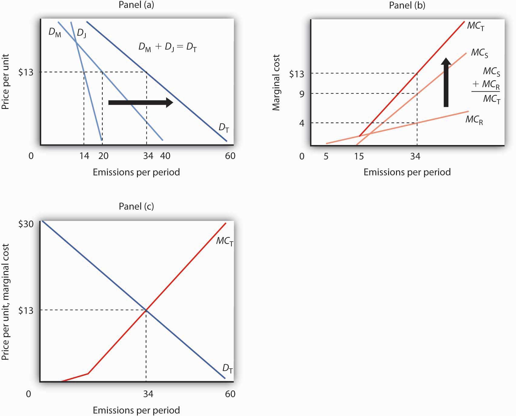
Mary and Jane each benefit from polluting the environment by emitting smoke from their fires. In Panel (a), we see that Mary’s demand curve for emitting smoke is given by DM and that Jane’s demand curve is given by DJ. To determine the total demand curve, DT, we determine the amount that each person will emit at various prices. At a price of $13 per day, for example, Mary will emit 20 pounds per day. Jane will emit 14 pounds per day, for a total of 34 pounds per day on demand curve DT. Notice that if the price were $0 per unit, Mary would emit 40 pounds per day, Jane would emit 20, and emissions would total 60 pounds per day on curve DT. The marginal cost curve for pollution is determined in Panel (b) by taking the marginal cost curves for each person affected by the pollution. In this case, the only people affected are Sam and Richard. Sam’s marginal cost curve is MCS, and Richard’s marginal cost curve is MCR. Because Sam and Richard are each affected by the same pollution, we add their marginal cost curves vertically. For example, if the total quantity of the emissions is 34 pounds per day, the marginal cost of the 34th pound to Richard is $4, it is $9 to Sam, for a total marginal cost of the 34th unit of $13. In Panel (c), we put DT and MCT together to find the efficient solution. The two curves intersect at a level of emissions of 34 pounds per day, which occurs at a price of $13 per pound.
Suppose, as is often the case, that no mechanism exists to charge Mary and Jane for their emissions; they can pollute all they want and never have to compensate society (that is, pay Sam and Richard) for the damage they do. Alternatively, suppose there is no mechanism for Sam and Richard to pay Mary and Jane to get them to reduce their pollution. In either situation, the pollution generated by Mary and Jane imposes an external cost on Sam and Richard. Mary and Jane will pollute up to the point that the marginal benefit of additional pollution to them has reached zero—that is, up to the point where the marginal benefit matches their marginal cost. They ignore the external costs they impose on “society”—Sam and Richard.
Mary’s and Jane’s demand curves for pollution are shown in Panel (a). These demand curves, DM and DJ, show the quantities of emissions each generates at each possible price, assuming such a fee were assessed. At a price of $13 per unit, for example, Mary will emit 20 units of pollutant per period and Jane will emit 14. Total emissions at a price of $13 would be 34 units per period. If the price of emissions were zero, total emissions would be 60 units per period. Whatever the price they face, Mary and Jane will emit additional units of the pollutant up to the point that their marginal benefit equals that price. We can therefore interpret their demand curves as their marginal benefit curves for emissions. Their combined demand curve DT gives the marginal benefit to society (that is, to Mary and Jane) of pollution. Each person in our problem, Mary, Jane, Sam, and Richard, follows the marginal decision rule and thus attempts to maximize utility.
In Panel (b) we see how much Sam and Richard are harmed; the marginal cost curves, MCS and MCR, show their respective valuations of the harm imposed on them by each additional unit of emissions. Notice that over a limited range, some emissions generate no harm. At very low levels, neither Sam nor Richard is even aware of the emissions. Richard begins to experience harm as the quantity of emissions goes above 5 pounds per day; it is here that pollution begins to occur. As emissions increase, the additional harm each unit creates becomes larger and larger—the marginal cost curves are upward sloping. The first traces of pollution may be only a minor inconvenience, but as pollution goes up, the problems it creates become more serious—and its marginal cost rises.
Because the same emissions affect both Sam and Richard, we add their marginal cost curves vertically to obtain their combined marginal cost curve MCT. The 34th unit of emissions, for example, imposes an additional cost of $9 on Sam and $4 on Richard. It thus imposes a total marginal cost of $13.
The efficient quantity of emissions is found at the intersection of the demand (DT) and marginal cost (MCT) curves in Panel (c) of Figure 18.1 “Determining the Efficient Level of Pollution”, with 34 units of the pollutant emitted. The marginal benefit of the 34th unit of emissions, as measured by the demand curve DT, equals its marginal cost, MCT, at that level. The quantity at which the marginal benefit curve intersects the marginal cost curve maximizes the net benefit of an activity.
We have already seen that in the absence of a mechanism to charge Mary and Jane for their emissions, they face a price of zero and would emit 60 units of pollutant per period. But that level of pollution is inefficient. Indeed, as long as the marginal cost of an additional unit of pollution exceeds its marginal benefit, as measured by the demand curve, there is too much pollution; the net benefit of emissions would be greater with a lower level of the activity.
Just as too much pollution is inefficient, so is too little. Suppose Mary and Jane are not allowed to pollute; emissions equal zero. We see in Panel (c) that the marginal benefit of dumping the first unit of pollution is quite high; the marginal cost it imposes on Sam and Richard is zero. Because the marginal benefit of additional pollution exceeds its marginal cost, the net benefit to society would be increased by increasing the level of pollution. That is true at any level of pollution below 34 units, the efficient solution.
The notion that too little pollution could be inefficient may strike you as strange. To see the logic of this idea, imagine that the pollutant involved is carbon monoxide, a pollutant emitted whenever combustion occurs, and it is deadly. It is, for example, emitted when you drive a car. Now suppose that no emissions of carbon monoxide are allowed. Among other things, this would require a ban on all driving. Surely the benefits of some driving would exceed the cost of the pollution created. The problem in pollution policy from an economic perspective is to find the quantity of pollution at which total benefits exceed total costs by the greatest possible amount—the solution at which marginal benefit equals marginal cost.
Property Rights and the Coase Theorem
The problem of getting the efficient amount of pollution arises because no one owns the right to the air. If someone did, then that owner could decide how to use it. If a nonowner did not like the way the owner was using it, then he or she could try to pay the owner to change the way the air was being used.
In our earlier example, if Mary and Jane own the right to the air, but Sam and Richard do not like how much Mary and Jane are polluting it, Sam and Richard can offer to pay Mary and Jane to cut back on the amount they are polluting. Alternatively, if Sam and Richard own the air, then in order to pollute it, Mary and Jane would have to compensate the owners. Bargaining among the affected parties, if costless, would lead to the efficient amount of pollution. Costless bargaining requires that all parties know the source of the pollution and are able to measure the quantity emitted by each agent.
Specifically, suppose Mary and Jane own the right to dump pollutants into the air and had been emitting 60 units of the pollution per day. If Sam and Richard offer to pay them $13 for each unit of pollutant they cut back, Mary and Jane will reduce their pollution to 34 units, since the marginal benefit to them of the 35th to 60th unit is less than $13. Sam and Richard are better off since the marginal cost of those last 26 units of pollution is greater than $13 per unit. The efficient outcome of 34 units of pollution is thus achieved. Mary and Jane could reduce their emissions by burning their fires for less time, by selecting more efficient fireplaces, or by other measures. Many people, for example, have reduced their emissions by changing to gas-burning fireplaces rather than burning wood.
While the well-being of the affected parties is not independent of who owns the property right (each would be better off owning rather than not owning the right), the establishment of who owns the air leads to a solution that solves the externality problem and leads to an efficient market outcome. The proposition that if property rights are well defined and if bargaining is costless, the private market can achieve an efficient outcome regardless of which of the affected parties holds the property rights is known as the Coase theorem, named for the Nobel-Prize-winning economist Ronald Coase who generally is credited with this idea.
Suppose instead that Sam and Richard own the right to the air. They could charge Mary and Jane $13 per unit of pollution emitted. Mary and Jane would willingly pay for the right to emit 34 units of pollution, but not for any more, since beyond that amount the marginal benefit of each unit of pollution emitted is less than $13. Sam and Richard would willingly accept payments for 34 units of pollution at $13 each since the marginal cost to them for each of those units is less than $13.
In most cases, however, Coase stressed that the conditions for private parties to achieve an efficient outcome on their own are not present. Property rights may not be defined. Even if one party owns a right, enforcement may be difficult. Suppose Sam and Richard own the right to clean air but many people, not just two as in our example, contribute to polluting it. Would each producer that pollutes have to strike a deal with Sam and Richard? Could the government enforce all those deals? And what if there are many owners as well? Enforcement becomes increasingly difficult and striking deals becomes more and more costly. Finally, monitoring is extremely difficult in most environmental problems. While it is generally possible to detect the presence of pollutants, determining their source is virtually impossible. And determining who is harmed and by how much is a monumental undertaking in most pollution problems.
Nonetheless, it is the insight that the Coase theorem provides that has led economists to consider solutions to environmental problems that attempt to use the establishment of property rights and market mechanisms in various ways to bring about the efficient market outcome. Before considering alternative ways of controlling pollution, we look first at how the benefits and costs might be measured so that we have a better sense of what the efficient solution is.
Another insight that comes from Coase’s analysis is that the notion of “harm” is a reciprocal one. In our first example, it is tempting to conclude that Mary and Jane, by burning fires in their fireplaces, are “harming” Sam and Richard. But if Sam and Richard were not located downwind of the smoke, there would be no harm. In effect, Mr. Coase insists that the harm cannot be attributed to one party or another. Sam and Richard “cause” the harm by locating downwind of the fireplaces. While there is clearly harm in this situation, we could as easily attribute it to either the generators of the smoke or the recipients of the smoke. Before Coase wrote his article, “The Problem of Social Cost” in 1960, the general presumption was that decision makers such as Mary and Jane “cause” the harm and that they should be taxed for the costs they impose. Mr. Coase pointed out the alternative that Sam and Richard could avoid the harm by moving. Indeed, all sorts of alternative solutions come to mind even in this simple example. Mary and Jane could select types of wood that emit less smoke. They could use fireplaces that emit less smoke. They could make arrangements to time their burning to minimize the total amount of smoke that affects Sam and Richard. The goal, Coase said, is to select the most efficient from the alternatives available (Coase, R. H., 1960).
Consider a different problem. Suppose that an airport has been built several miles outside the developed portion of a small city. No one lives close enough to the airport to be “harmed” by the noise inevitably generated by the operation of the airport. As time passes, people are likely to build houses near the airport to take advantage of jobs at the airport or to gain easy access to it. Those people will now be “harmed” by noise from the airport. But what is the cause of this harm? By definition, there was no “harm” before people started living close to the airport. True, it is the airport that generates the noise. But the noise causes harm only because people now live near it. Just as Mary and Jane’s campfires only generate “harm” if someone is downwind of the smoke, the noise from the airport causes damage only if someone lives near the airport. The problem of the noise could be mitigated in several ways. First, people could have chosen not to live near the airport. Once they have chosen to live near the airport, they could reduce the noise with better insulation or with better windows. Alternatively, the airport management could choose different flight patterns to reduce noise that affects neighboring homeowners. It is always the case that there are several potential ways of mitigating the effects of airport operations; the economic problem is to select the most efficient from among those alternatives.
The Measurement of Benefits and Costs
Saying that the efficient level of pollution occurs at a certain rate of emissions, as we have done so far, is one thing. Determining the actual positions of the demand and marginal cost curves that define that efficient solution is quite another. Economists have devised a variety of methods for measuring these curves.
Benefits: The Demand for Emissions
A demand curve for emitting pollutants shows the quantity of emissions demanded per unit of time at each price. It can, as we have seen, be taken as a marginal benefit curve for emitting pollutants.
The general approach to estimating demand curves involves observing quantities demanded at various prices, together with the values of other determinants of demand. In most pollution problems, however, the price charged for emitting pollutants has always been zero—we simply do not know how the quantity of emissions demanded will vary with price.
One approach to estimating the demand curve for pollution utilizes the fact that this demand occurs because pollution makes other activities cheaper. If we know how much the emission of one more unit of a pollutant saves, then we can infer how much consumers or firms would pay to dump it.
Suppose, for example, that there is no program to control automobile emissions—motorists face a price of zero for each unit of pollution their cars emit. Suppose that a particular motorist’s car emits an average of 10 pounds of carbon monoxide per week. Its owner could reduce emissions to 9 pounds per week at a cost of $1 per week. This $1 is the marginal cost of reducing emissions from 10 to 9 pounds per week. It is also the maximum price the motorist would pay to increase emissions from 9 to 10 pounds per week—it is the marginal benefit of the 10th pound of pollution. We say that it is the maximum price because if asked to pay more, the motorist would choose to reduce emissions at a cost of $1 instead.
Now suppose that emissions have been reduced to 9 pounds per week and that the motorist could reduce them to 8 at an additional cost of $2 per week. The marginal cost of reducing emissions from 9 to 8 pounds per week is $2. Alternatively, this is the maximum price the motorist would be willing to pay to increase emissions to 9 from 8 pounds; it is the marginal benefit of the 9th pound of pollution. Again, if asked to pay more than $2, the motorist would choose to reduce emissions to 8 pounds per week instead.
Figure 18.2 Abatement Costs and Demand
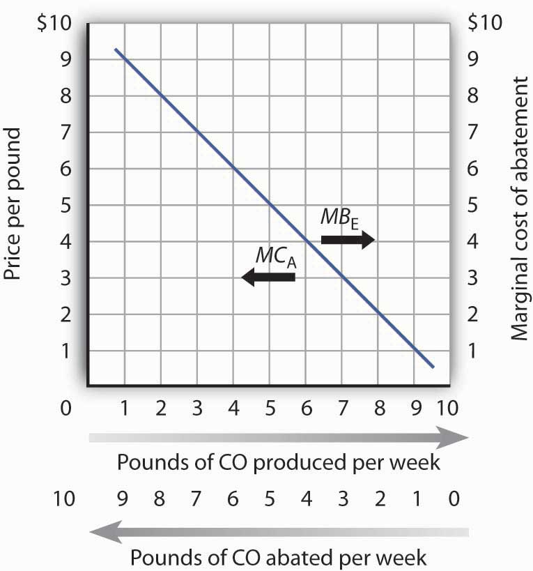
A car emits an average of 10 pounds of CO per week when no restrictions are imposed—when the price of emissions is zero. The marginal cost of abatement (MCA) is the cost of eliminating a unit of emissions; this is the interpretation of the curve when read from right to left. The same curve can be read from left to right as the marginal benefit of emissions (MBE).
We can thus think of the marginal benefit of an additional unit of pollution as the added cost of not emitting it. It is the saving a polluter enjoys by dumping additional pollution rather than paying the cost of preventing its emission. Figure 18.2 “Abatement Costs and Demand” shows this dual interpretation of cost and benefit. Initially, our motorist emits 10 pounds of carbon monoxide per week. Reading from right to left, the curve measures the marginal costs of pollution abatement (MCA). We see that the marginal cost of abatement rises as emissions are reduced. That makes sense; the first reductions in emissions will be achieved through relatively simple measures such as modifying one’s driving technique to minimize emissions (such as accelerating more slowly), or getting tune-ups more often. Further reductions, however, might require burning more expensive fuels or installing more expensive pollution-control equipment.
Read from left to right, the curve in Figure 18.2 “Abatement Costs and Demand” shows the marginal benefit of additional emissions (MBE). Its negative slope suggests that the first units of pollution emitted have very high marginal benefits, because the cost of not emitting them would be very high. As more of a pollutant is emitted, however, its marginal benefit falls—the cost of preventing these units of pollution becomes quite low.
Economists have also measured demand curves for emissions by using surveys in which polluters are asked to report the costs to them of reducing their emissions. In cases in which polluters are charged for the emissions they create, the marginal benefit curve can be observed directly.
As we saw in Figure 18.1 “Determining the Efficient Level of Pollution”, the marginal benefit curves of individual polluters are added horizontally to obtain a market demand curve for pollution. This curve measures the additional benefit to society of each additional unit of pollution.
The Marginal Cost of Emissions
Pollutants harm people and the resources they value. The marginal cost curve for a pollutant shows the additional cost imposed by each unit of the pollutant. As we saw in Figure 18.1 “Determining the Efficient Level of Pollution”, the marginal cost curves for all the individuals harmed by a particular pollutant are added vertically to obtain the marginal cost curve for the pollutant.
Like the marginal benefit curve for emissions, the marginal cost curve can be interpreted in two ways, as suggested in Figure 18.3 “The Marginal Cost of Emissions and the Marginal Benefit of Abatement”. When read from left to right, the curve measures the marginal cost of additional units of emissions (MCE). If increasing the motorists’ emissions from four pounds of carbon monoxide per week to five pounds of carbon monoxide per week imposes an external cost of $2, though, the marginal benefit of not being exposed to that unit of pollutant must be $2. The marginal cost curve can thus be read from right to left as a marginal benefit curve for abating emissions (MBA). This marginal benefit curve is, in effect, the demand curve for cleaner air.
Figure 18.3 The Marginal Cost of Emissions and the Marginal Benefit of Abatement
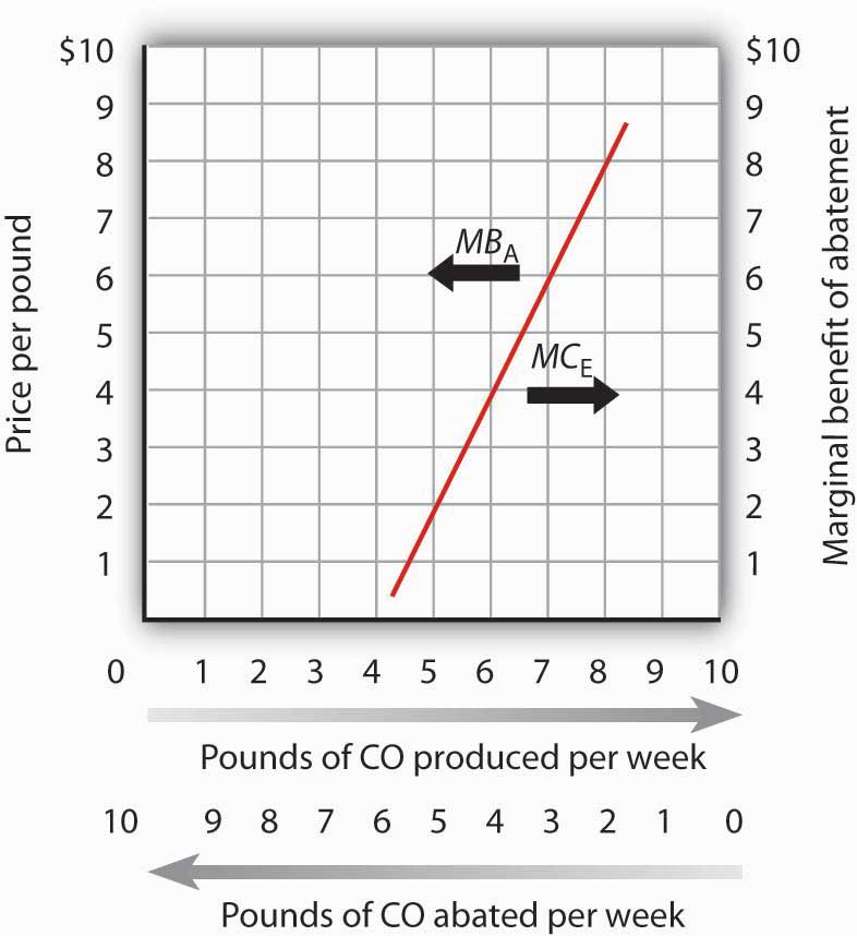
The marginal cost of the first few units of emissions is zero and then rises once emissions begin to harm people. That is the point at which the air becomes a scarce resource. Read from left to right the curve gives the marginal cost of emissions (MCE). Read from right to left, the curve gives the marginal benefit of abatement (MBA).
Economists estimate the marginal cost curve of pollution in several ways. One is to infer it from the demand for goods for which environmental quality is a complement. Another is to survey people, asking them what pollution costs—or what they would pay to reduce it. Still another is to determine the costs of damages created by pollution directly.
For example, environmental quality is a complement of housing. The demand for houses in areas with cleaner air is greater than the demand for houses in areas that are more polluted. By observing the relationship between house prices and air quality, economists can learn the value people place on cleaner air—and thus the cost of dirtier air. Studies have been conducted in cities all over the world to determine the relationship between air quality and house prices so that a measure of the demand for cleaner air can be made. They show that increased pollution levels result in lower house values (Becker, N. and Doron Laee, 2003).
Surveys are also used to assess the marginal cost of emissions. The fact that the marginal cost of an additional unit of emissions is the marginal benefit of avoiding the emissions suggests that surveys can be designed in two ways. Respondents can be asked how much they would be harmed by an increase in emissions, or they can be asked what they would pay for a reduction in emissions. Economists often use both kinds of questions in surveys designed to determine marginal costs.
A third kind of cost estimate is based on objects damaged by pollution. Increases in pollution, for example, require buildings to be painted more often; the increased cost of painting is one measure of the cost of added pollution.
While all of the attempts to measure cost are imperfect, the alternative is to not try to quantify cost at all. To economists, such an ostrich-like approach of sticking one’s head in the sand would be unacceptable.
The Efficient Level of Emissions and Abatement
Whether economists measure the marginal benefits and marginal costs of emissions or, alternatively, the marginal benefits and marginal costs of abatement, the policy implications are the same from an economic perspective. As shown in Panel (a) of Figure 18.4 “The Efficient Level of Emissions and Pollution Abatement”, applying the marginal decision rule in the case of emissions suggests that the efficient level of pollution occurs at six pounds of CO emitted per week. At any lower level, the marginal benefits of the pollution would outweigh the marginal costs. At a higher level, the marginal costs of the pollution would outweigh the marginal benefits.
Figure 18.4 The Efficient Level of Emissions and Pollution Abatement
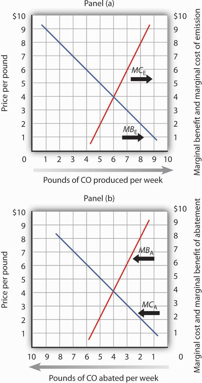
In Panel (a) we combine the marginal benefit of emissions (MBE) with the marginal cost of emissions (MCE). The efficient solution occurs at the intersection of the two curves. Here, the efficient quantity of emissions is six pounds of CO per week. In Panel (b), we have the same curves read from right to left. The marginal cost curve for emissions becomes the marginal benefit of abatement (MBA). The marginal benefit curve for emissions becomes the marginal cost of abatement (MCA). With no abatement program, emissions total ten pounds of CO per week. The efficient degree of abatement is to reduce emissions by four pounds of CO per week to six pounds per week.
As shown in Panel (b) of Figure 18.4 “The Efficient Level of Emissions and Pollution Abatement”, application of the marginal decision rule suggests that the efficient level of abatement effort is to reduce pollution by 4 pounds of CO produced per week. That is, reduce the level of pollution from the 10 pounds per week that would occur at a zero price to 6 pounds per week. For any greater effort at abating the pollution, the marginal cost of the abatement efforts would exceed the marginal benefit.
Key Takeaways
- Pollution is related to the concept of scarcity. The existence of pollution implies that an environmental resource has alternative uses and is thus scarce.
- Pollution has benefits as well as costs; the emission of pollutants benefits people by allowing other activities to be pursued at lower costs. The efficient rate of emissions occurs where the marginal benefit of emissions equals the marginal cost they impose.
- The marginal benefit curve for emitting pollutants can also be read from right to left as the marginal cost of abating emissions. The marginal cost curve for increased emission levels can also be read from right to left as the demand curve for improved environmental quality.
- The Coase theorem suggests that if property rights are well-defined and if transactions are costless, then the private market will reach an efficient solution. These conditions, however, are not likely to be present in typical environmental situations. Even if such conditions do not exist, Coase’s arguments still yield useful insights to the mitigation of environmental problems.
- Surveys are sometimes used to measure the marginal benefit curves for emissions and the marginal cost curves for increased pollution levels. Marginal cost curves may also be inferred from other relationships. Two that are commonly used are the demand for housing and the relationship between pollution and production.
Try It!
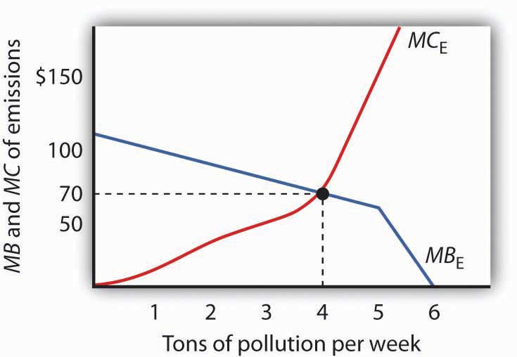
The table shows the marginal benefit to a paper mill of polluting a river and the marginal cost to residents who live downstream. In this problem assume that the marginal benefits and marginal costs are measured at (not between) the specific quantities shown.
Plot the marginal benefit and marginal cost curves. What is the efficient quantity of pollution? Explain why neither one ton nor five tons is an efficient quantity of pollution. In the absence of pollution fees or taxes, how many units of pollution do you expect the paper mill will choose to produce? Why?
|
Quantity of pollution (tons per week) |
Marginal benefit | Marginal cost |
|---|---|---|
| 0 | $110 | $0 |
| 1 | 100 | 8 |
| 2 | 90 | 20 |
| 3 | 80 | 35 |
| 4 | 70 | 70 |
| 5 | 60 | 150 |
| 6 | 0 | 300 |
Case in Point: Estimating a Demand Curve for Environmental Quality

How do economists estimate demand curves for environmental quality? One recent example comes from work by Louisiana State University economist David M. Brasington and Auburn University economist Diane Hite. Using data from Ohio’s six major metropolitan areas (Akron, Cincinnati, Cleveland, Columbus, Dayton, and Toledo), the economists studied the relationship between house prices and the distance between individual houses and hazardous waste sites. From this, they were able to estimate the demand curve for environmental quality—at least in terms of the demand for locations farther from environmental hazards.
The economists used actual real estate transactions in 1991 to get data on house prices. In that year, there were 1,192 hazardous sites in the six metropolitan areas. The study was based on 44,255 houses. The median distance between a house and a hazardous site was 1.08 miles. The two economists found, as one would expect, that house prices were higher the greater the distance between the house and a hazardous site. All other variables unchanged, increasing the distance from a house to a hazardous site by 10% increased house value by 0.3%.
Other characteristics of the demand curve shed light on the relationship between environmental quality and other goods. For example, the study showed that people substitute house size for environmental quality. A house closer to a hazardous waste site is cheaper; people take advantage of the lower price of such sites to purchase larger houses.
While house size and environmental quality were substitutes, school quality, measured by student scores on achievement tests, was a complement. If the price of school quality were to fall by 10%, household would buy 8% more environmental quality. The cross-price elasticity between environmental quality and school quality was thus estimated to be −0.80.
There is no marketplace for environmental quality. Estimating the demand curve for such quality requires economists to examine other data to try to infer what the demand curve is. The study by Professors Brasington and Hite illustrates the use of an examination of an actual market, the market for houses, to determine characteristics of the demand curve for environmental quality.
Source: David M. Brasington and Diane Hite, “Demand for Environmental Quality: A Spatial Hedonic Analysis,” Regional Science & Urban Economics, 35(1) (January 2005): 57–82.
Answer to Try It! Problem
The efficient quantity of pollution is four tons per week. At one ton of pollution, the marginal benefit exceeds the marginal cost. If the paper mill expands production, the additional pollution generated leads to additional benefits for it that are greater than the additional cost to the residents nearby. At five tons, the marginal cost of polluting exceeds the marginal benefit. Reducing production, and hence pollution, brings the marginal costs and benefits closer.
In the absence of any fees, taxes, or other charges for its pollution, the paper mill will likely choose to generate six tons per week, where the marginal benefit has fallen to zero.
Figure 18.6
References
Becker, N., and Doron Lavee, “The Benefits and Costs of Noise Reduction,” Journal of Environmental Planning and Management, 46(1) (January 2003): 97–111, which shows the negative relationship between apartment prices and noise levels (a form of pollution) in Israel.
Coase, R. H., “The Problem of Social Cost,” Journal of Law and Economics 3 (October 1960): 1–44.
