13.4 Review and Practice
Summary
This chapter presented the aggregate expenditures model. Aggregate expenditures are the sum of planned levels of consumption, investment, government purchases, and net exports at a given price level. The aggregate expenditures model relates aggregate expenditures to the level of real GDP.
We began by observing the close relationship between consumption and disposable personal income. A consumption function shows this relationship. The saving function can be derived from the consumption function.
The time period over which income is considered to be a determinant of consumption is important. The current income hypothesis holds that consumption in one period is a function of income in that same period. The permanent income hypothesis holds that consumption in a period is a function of permanent income. An important implication of the permanent income hypothesis is that the marginal propensity to consume will be smaller for temporary than for permanent changes in disposable personal income.
Changes in real wealth and consumer expectations can affect the consumption function. Such changes shift the curve relating consumption to disposable personal income, the graphical representation of the consumption function; changes in disposable personal income do not shift the curve but cause movements along it.
An aggregate expenditures curve shows total planned expenditures at each level of real GDP. This curve is used in the aggregate expenditures model to determine the equilibrium real GDP (at a given price level). A change in autonomous aggregate expenditures produces a multiplier effect that leads to a larger change in equilibrium real GDP. In a simplified economy, with only consumption and investment expenditures, in which the slope of the aggregate expenditures curve is the marginal propensity to consume (MPC), the multiplier is equal to 1/(1 − MPC). Because the sum of the marginal propensity to consume and the marginal propensity to save (MPS) is 1, the multiplier in this simplified model is also equal to 1/MPS.
Finally, we derived the aggregate demand curve from the aggregate expenditures model. Each point on the aggregate demand curve corresponds to the equilibrium level of real GDP as derived in the aggregate expenditures model for each price level. The downward slope of the aggregate demand curve (and the shifting of the aggregate expenditures curve at each price level) reflects the wealth effect, the interest rate effect, and the international trade effect. A change in autonomous aggregate expenditures shifts the aggregate demand curve by an amount equal to the change in autonomous aggregate expenditures times the multiplier.
In a more realistic aggregate expenditures model that includes all four components of aggregate expenditures (consumption, investment, government purchases, and net exports), the slope of the aggregate expenditures curve shows the additional aggregate expenditures induced by increases in real GDP, and the size of the multiplier depends on the slope of the aggregate expenditures curve. The steeper the aggregate expenditures curve, the larger the multiplier; the flatter the aggregate expenditures curve, the smaller the multiplier.
Concept Problems
- Explain the difference between autonomous and induced expenditures. Give examples of each.
- The consumption function we studied in the chapter predicted that consumption would sometimes exceed disposable personal income. How could this be?
- The consumption function can be represented as a table, as an equation, or as a curve. Distinguish among these three representations.
- The introduction to this chapter described the behavior of consumer spending at the end of 2008. Explain this phenomenon in terms of the analysis presented in this chapter.
- Explain the role played by the 45-degree line in the aggregate expenditures model.
- Your college or university, if it does what many others do, occasionally releases a news story claiming that its impact on the total employment in the local economy is understated by its own employment statistics. If the institution keeps accurate statistics, is that possible?
- Suppose the level of investment in a certain economy changes when the level of real GDP changes; an increase in real GDP induces an increase in investment, while a reduction in real GDP causes investment to fall. How do you think such behavior would affect the slope of the aggregate expenditures curve? The multiplier?
- Give an intuitive explanation for how the multiplier works on a reduction in autonomous aggregate expenditures. Why does equilibrium real GDP fall by more than the change in autonomous aggregate expenditures?
- Explain why the marginal propensity to consume out of a temporary tax rebate would be lower than that for a permanent rebate.
- Pretend you are a member of the Council of Economic Advisers and are trying to persuade the members of the House Appropriations Committee to purchase $100 billion worth of new materials, in part to stimulate the economy. Explain to the members how the multiplier process will work.
Numerical Problems
- Suppose the following information describes a simple economy. Figures are in billion of dollars.
Disposable personal income Consumption 0 100 100 120 200 140 300 160 - What is the marginal propensity to consume?
- What is the marginal propensity to save?
- Write an equation that describes consumption.
- Write an equation that describes saving.
- The graph below shows a consumption function.
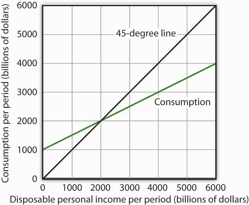
- When disposable personal income is equal to zero, how much is consumption?
- When disposable personal income is equal to $4,000 billion, how much is consumption?
- At what level of personal disposable income are consumption and disposable personal income equal?
- How much is personal saving when consumption is $2,500 billion?
- How much is personal saving when consumption is $5,000 billion?
- What is the marginal propensity to consume?
- What is the marginal propensity to save?
- Draw the saving function implied by the consumption function above.
- For the purpose of this exercise, assume that the consumption function is given by C = $500 billion + 0.8Yd. Construct a consumption and saving table showing how income is divided between consumption and personal saving when disposable personal income (in billions) is $0, $500, $1,000, $1,500, $2,000, $2,500, $3,000, and $3,500.
- Graph your results, placing disposable personal income on the horizontal axis and consumption on the vertical axis.
- What is the value of the marginal propensity to consume?
- What is the value of the marginal propensity to save?
- The graph below characterizes a simple economy with only two components of aggregate expenditures, consumption and investment.
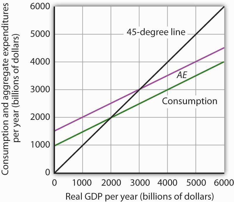
- How much is planned investment? How do you know?
- Is planned investment autonomous or induced? How do you know?
- How much is autonomous aggregate expenditures?
- What is the value of equilibrium real GDP?
- If real GDP were $2,000 billion, how much would unplanned investment be? How would you expect firms to respond?
- If real GDP were $4,000 billion, how much would unplanned investment be? How would you expect firms to respond?
- Write an equation for aggregate expenditures based on the graph above.
- What is the value of the multiplier in this example?
- Explain and illustrate graphically how each of the following events affects aggregate expenditures and equilibrium real GDP. In each case, state the nature of the change in aggregate expenditures, and state the relationship between the change in AE and the change in equilibrium real GDP.
- Investment falls.
- Government purchases go up.
- The government sends $1,000 to every person in the United States.
- Real GDP rises by $500 billion.
- Mary Smith, whose marginal propensity to consume is 0.75, is faced with an unexpected increase in taxes of $1,000. Will she cut back her consumption expenditures by the full $1,000? How will she pay for the higher tax? Explain.
- The equations below give consumption functions for economies in which planned investment is autonomous and is the only other component of GDP. Compute the marginal propensity to consume and the multiplier for each economy.
- C = $650 + 0.33Y
- C = $180 + 0.9Y
- C = $1,500
- C = $700 + 0.8Y
- Suppose that in Economies A and B the only components of aggregate expenditure are consumption and planned investment. The marginal propensity to consume in Economy A is 0.9, while in Economy B it is 0.7. Both economies experience an increase in planned investment, which is assumed to be autonomous, of $100 billion. Compare the changes in the equilibrium level of real GDP and the shifts in aggregate demand this will produce in the two economies.
- Assume an economy in which people would spend $200 billion on consumption even if real GDP were zero and, in addition, increase their consumption by $0.50 for each additional $1 of real GDP. Assume further that the sum of planned investment plus government purchases plus net exports is $200 billion regardless of the level of real GDP.
- What is the equilibrium level of income in this economy?
- If the economy is currently operating at an output level of $1,200 billion, what do you predict will happen to real GDP in the future?
- Suppose the aggregate expenditures curve in Numerical Problem 9 is drawn for a price level of 1.2. A reduction in the price level to 1 increases aggregate expenditures by $400 billion at each level of real GDP. Draw the implied aggregate demand curve.


