14.3 Linkage and Inheritance of Small Differences
Learning objectives
By the end of this section you will:
- Know the meaning of linkage and the impact of crossing over on linked loci.
- Recognize the difference between qualitative and quantitative inheritance.
- Understand how heritability is a measure of the genetic influence over a quantitative trait, relative to other non-genetic influences.
Review
The previous section included examples of simple inheritance, where large, obvious, discrete differences among plants are controlled by one gene and where one of the alleles is completely dominant over the other. Based on the inheritance patterns of round vs. wrinkled pea seeds described in that lesson, Mendel developed the Law of Segregation.
Often called Mendel’s First Law, the Law of Segregation in modern terms states that, during gamete formation, the two alleles for the gene of interest (recall that in diploid cells there are two homologs for each type of chromosome, so there are potentially two versions or alleles of each gene) separate from each other during meiosis and are passed individually to the next generation through the egg and sperm. This is apparent in the mechanics of meiosis, where the homologs separate and migrate to opposite poles in Anaphase I and, following the separation of sister chromatids in Anaphase II, are packaged into separate gametes. In the self-pollination of a Smooth x Wrinkled F1 pea example, the Ss diploid produces S and s gametes, not Ss gametes. The S and s are segregated into separate gametes.
The previous lesson also tracked the joint inheritance of two genes on separate chromosomes that affect different traits (Smooth vs Wrinkled seeds and Yellow vs Green seeds), which leads to Mendel’s Second Law — the Law of Independent Assortment. In modern terms, this law roughly states that, during gamete formation, the allocation of the alleles of a gene on one chromosome is independent of the allocation of the alleles of a different gene on a different (non-homologous) chromosome. So when gametes form from an SsYy F1, and the gametes receive either S or s (as stated in the First Law of Segregation), then whether Y goes with S to make up a SY gamete, or whether y goes with S to make up a Sy gamete, is completely by chance. This is also seen in the diagram of meiosis and how the chromosomes divide at Anaphase I. Homologs separate at Anaphase I, and in the case of two different pairs of homologs, the way in which the first pair of homologs splits doesn’t influence how the second pair of homologs splits. What Mendel discovered by examining segregation ratios (the ratios of each genotype resulting from a particular cross) can thus also be explained through the mechanics of meiosis. Mendel’s thinking was revolutionary at the time, and a great example of thinking carefully about the outcomes of an experiment and developing a model of the process that explains the observed data.
Linkage
Watch this video for an explanation of linkage (7:47)
What if those two genes are positioned closely on the same chromosome rather than on separate chromosomes, as in the pea shape/pea color example? This situation is called linkage.
Imagine a case in which the hypothetical gene “A” (with alleles “A” and “a“) and gene “B” (with alleles “B” and “b“) occur at loci near each other on the same chromosome. Imagine further that one of the chromosomes has the dominant “A” and the dominant “B” allele while its homolog has both recessive “a” and “b” alleles. This situation is illustrated below.
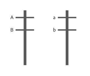
When these chromosomes go through meiosis the alleles at the two loci cannot independently assort because they are on the same chromosome — they are physically connected. As a result, the gametes will be either AB or ab. There will be no Ab or aB gametes, as you would normally expect from independent assortment, because the A allele is physically attached to the B allele, and the a allele attached to the b allele — they are on the same chromosome. The only way to get Ab or aB gametes together is through a physical breakage in the chromosomes between the two genes and the exchange of arms between homologs; recall that this is called crossing over.
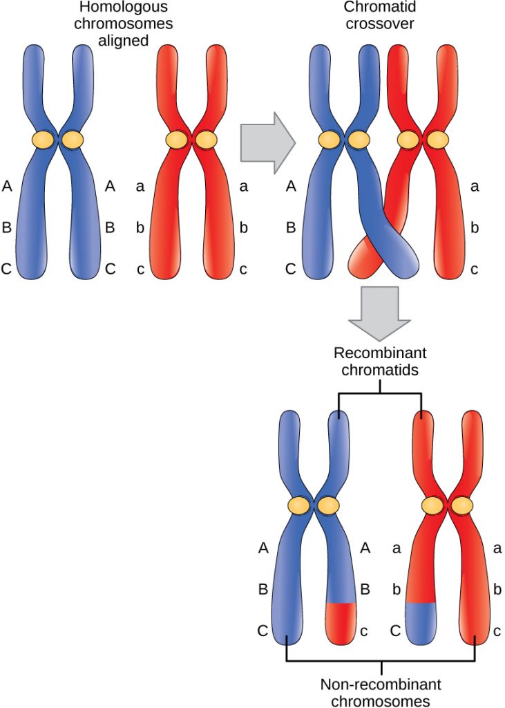
The illustration shows homologs in Prophase I following synapsis (pairing) and where sister chromatids crossed over, with the cross-over event occurring between the loci for the two genes. The chromatids cross over and will exchange arms. When they separate at Anaphase I, the homolog that migrates to the left side will have one sister chromatid with the alleles AB and one with aB. The homolog that migrates to the right will have one chromatid that is Ab and another that is ab.
The frequency of crossing over is one way to describe the distance between the two genes on the chromosome. If crossing over is very infrequent — in this example, if there are very few Ab and aB gametes — the two genes must be very close to each other. This situation is called a tight linkage. If crossing over is quite frequent, approaching 50%, the two genes must be very far apart. If it appears that AB, ab, Ab, and aB gametes have equal frequency, this indicates that the genes are located on different chromosomes or are on the same chromosome, but separated so much that the frequency of crossing over is 50%, which has the same result as if they were on separate chromosomes.
The Wikipedia site on linkage provides a bit of additional information.
Review questions
- Why can two linked genes NOT independently assort?
- In the example above, will tight linkage result in many or few Ab gametes?
- Would you expect the frequency of aB gametes to be roughly the same or quite different from the frequency of Ab gametes?
Quantitative traits — inheritance of small differences
Watch this video for an introduction to quantitative traits (8:28)
Recall that inheritance does not always involve large, qualitative differences. Inheritance of small differences that require more meticulous measurement and are reported in quantitative terms such as seed yield in kg/ha, number of chloroplasts per mesophyll cell, and grape sucrose content are very important in horticulture. Indeed, these small differences, when accumulated, can be more important than the large qualitative differences in horticultural food crops. Quantitative traits result in higher yield, earlier maturity, and greater cold tolerance, all of which, with patient intercrossing and persistent selection over many years, leads to continuous crop improvement.
In contrast to qualitative traits, the inheritance of quantitative traits may be influenced substantially by the environment. Recall the equation
Phenotype = Genotype + Environment
For quantitative traits, the Genotype component, or the influence of each of these quantitative genes, is quite small, and the influence of the Environment can be large relative to the contribution of Genotype.
You can visualize the difference between quantitative and qualitative inheritance by measuring a large set of plants of the same species (we’ll call it a population of plants) for a particular characteristic (we’ll use flower number per plant as an example). Using that data set containing flower numbers for a large number of plants, you can
- count the number of plants in the population that have one flower,
- count the number of plants with two flowers,
- count the number of plants with three flowers, and so on,
then calculate the frequency of each of these flower number classes in the population by dividing the number of plants with one flower by the total number of plants in the population, and so on for each of your flower number classes.
Next, you can make a graph plotting the flower number on the X axis against the frequency of plants with that flower number on the Y axis, giving a figure called a frequency distribution.
As an example, below are two databases containing hypothetical flower number data taken on 60 plants in two different populations. The first table is a hypothetical database illustrating what the population structure might look like if flower number was controlled by quantitative inheritance, and the second illustrates what the population might look like if flower number was controlled by qualitative inheritance. Both tables have three columns; the first shows the number of flowers, ranging from 1 to 15 per plant; the second shows the number of plants in the sample of 60 with the corresponding number of flowers; and the third shows the frequency of plants in the sample with the corresponding number of flowers per plant. In the quantitative database on the left, in the row corresponding to plants with four flowers, read across to see that there were two of these plants, and that their frequency was 2/60 = 0.0333, rounded to 0.03. This is called a frequency distribution table because it shows the frequency of plants with a particular class of a characteristic, in this case flower number per plant.
Notice that the frequencies in the quantitative table are spread out over a wide range of flower numbers, with a peak around seven flowers per plant. In the qualitative table, in contrast, the frequencies are clustered around two discrete flower numbers, with one large peak at about five flowers and a smaller peak at 13.
| Quantitative example | Qualitative example | |||||
| # Flowers | # Plants | Frequency | # Flowers | # Plants | Frequency | |
| 1 | 0 | 0 | 1 | 0 | 0 | |
| 2 | 0 | 0 | 2 | 0 | 0 | |
| 3 | 1 | .02 | 3 | 0 | 0 | |
| 4 | 2 | .03 | 4 | 3 | .05 | |
| 5 | 5 | .08 | 5 | 30 | .50 | |
| 6 | 7 | .12 | 6 | 9 | .15 | |
| 7 | 16 | .27 | 7 | 3 | .05 | |
| 8 | 15 | .25 | 8 | 0 | 0 | |
| 9 | 6 | .10 | 9 | 0 | 0 | |
| 10 | 4 | .07 | 10 | 0 | 0 | |
| 11 | 2 | .03 | 11 | 1 | .02 | |
| 12 | 2 | .03 | 12 | 1 | .02 | |
| 13 | 0 | 0 | 13 | 12 | .20 | |
| 14 | 0 | 0 | 14 | 1 | .02 | |
| 15 | 0 | 0 | 15 | 0 | 0 | |
| Total | 60 | 1.0 | Total | 60 | 1.0 |
These data are easier to understand in a graph, with the flower number on the X axis and the frequencies on the Y axis:
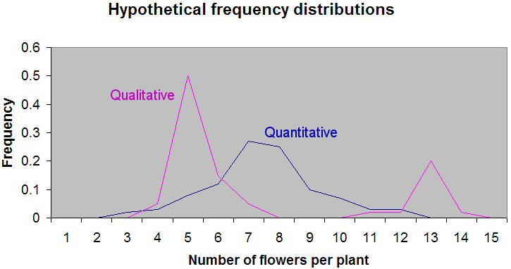
Notice that the magenta line illustrating the qualitative inheritance distribution has two peaks at 5 and 13 flowers per plant, and that the dispersion around those peaks is quite narrow. Most values are either 5 or 13. In contrast, the blue line illustrating quantitative inheritance has a peak in the 7–8 flower per plant region, and there is a great deal of dispersion. There are many different values of flowers per plant, although the most frequent is in the 7–8 range.
The dispersion around the peaks is in part due to the influence of the environment. For qualitative traits (magenta line), this influence is small. For quantitative traits (blue line), it is larger. Also notice that if you added up the frequencies under the two magenta curves, you would find that the curve with the peak at five flowers has three times the frequency of plants as the curve peaking at 13 plants. This 3:1 ratio is indicative of a single qualitative gene where the dominant allele is associated with, on average, five flowers per plant.
Review questions
- Would you expect that a frequency distribution with two sharp peaks represents a qualitative or quantitative trait?
- Would you expect that a frequency distribution which looks like a mound with one high point represents a qualitative or quantitative trait?
- Would you expect that a frequency distribution with four sharp peaks represents a qualitative or quantitative trait? (hint: 9:3:3:1)
Heritability
Watch this video for an introduction to heritability (8:44)
Inheritance of quantitative traits is often associated with the term heritability. If a parent and its offspring have very similar values for a quantitative trait, the trait is considered to be highly heritable. Highly heritable traits tend to be under strong genetic control with little influence from the environment. In contrast, if the offspring values don’t seem to have any relationship to that of the parent, the trait is considered to have low heritability. Low heritability usually results when the influence of the environment is quite high relative to the impact of the genotype on the trait being studied. If you are trying to improve a plant characteristic through breeding, you’ll have much greater gain from selection if the trait has high heritability rather than low heritability. If a plant characteristic has high heritability, dramatic changes to the population from natural selection will also be more rapid (require fewer generations) than for a characteristic that has low heritability. See the graph below.
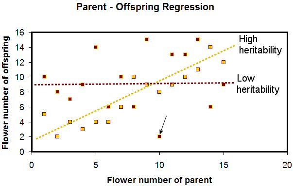
The X axis represents the number of flowers on the parent plant, while the Y axis represents the average number of flowers on the offspring of those parents. A dot represents each parent-offspring data pair. For example, the maroon dot with the black arrow pointing to it represents a data point for a parent with 10 flowers whose offspring had, on average, two flowers (read the 2 off the Y axis).
The gold dots represent cases where the trait has high heritability. Note that you can draw a line with a positive slope through the gold dots, with the dots being relatively close to the line. This indicates high heritability, and means that the offspring’s performance can be predicted based on the performance of the parent. If the parent has a high flower number, the offspring will as well. Plant breeders can make selections with the expectation that if they save seeds from superior plants, the offspring growing from those plants will exhibit the same superiority.
The maroon dots, in contrast, represent the situation of low or zero heritability, and have no line of good fit. Some parents with high flower numbers had offspring with low flower numbers and others with high flower numbers had offspring with high numbers. You can’t predict the offspring flower numbers based on the parent flower numbers. This represents a nightmare for breeders. Some offspring of superior plants will be good as the parents, others will be better, and others will be wildly inferior.
Review questions
- Would a breeder anticipate making greater gain from selection for a trait that has high heritability or low heritability?
- If a characteristic is very heavily influenced by the environment and exhibits very little control by genotype, will the heritability be close to 0 (very low heritability) or close to 1 (very high heritability)?
When two genes are on the same chromosome.
Measurement of a quantitative trait that passes from parent to offspring and is measured in high and low; high being very similar between parent and offspring and low being dissimilar between parent and offspring.
