7.7 Software and Technology Exercise

How to Set Up a Spreadsheet to Show Cash Flow, Simple Payback, and Calculate IRR

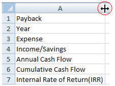
1. Start Excel 2007. In cells A1 through A5, type Payback and Internal Rate of Return, Year, Expense, Income/Savings, Annual Cash Flow, Cumulative Cash Flow, and Internal Rate of Return (IRR). Drag the boundary between column A and B to the right to increase the width of column A, as shown in Figure 7.14 “Widen Column to Fit Labels”.

   Figure 7.14 Widen Column to Fit Labels

   

2. In cell B2, type 0, and in cell C2, type 1. Click and drag across cells B2 and C2 to select them both. Identify the fill handle at the lower right corner of C2 as shown in Figure 7.15 “Use Fill Handle to Extend a Pattern of Intervals”. Selecting the first two numbers in a sequence determines the interval of the sequence.
3. Click and drag the fill handle to the right to cell H2. The sequence of years from zero to six is filled into cells B2 through H2.
4. In cell B3, type $(100,000) and then press the Enter key. Typing a number with the dollar sign and comma sets the formatting automatically. The parentheses indicate a negative number that the computer may display in red.
5. In cell C3, type $(2,000) and then press Enter. Click cell C3 again to select it. Drag the fill handle to the right to cell H3. Because a single value was selected, the same value is filled into cells D3 through H3, as shown in Figure 7.16 “Initial Expense in Year Zero Followed by Annual Expenses”.
6. In cell C4, type 25,000 and then press Enter. Use the procedure you practiced in step 5 to fill this value into cells D4 through H4.
7. In cell B5, type =B4+B3 and then press Enter. This formula adds the positive and negative cash flows in the two cells above its location to find the annual cash flow.
8. Click cell B5 and then drag the fill handle to cell H5 to fill this formula into the adjacent cells. The formulas adapt to their new locations to add the two cells immediately above. Click cell D5 to observe how the formulas change to sum the cells above, as shown in Figure 7.17 “Formula to Calculate a Running Total”.
9. In cell B6, type =B5 and then press Enter. This formula transfers the value for the initial expense to cell B6 so the next formula can be used in the remaining cells.
10. In cell C6, type =B6+C5 and then press Enter. This formula sums the value from the previous year with the annual cash flow for the current year.
11. Click cell C6 and then drag the fill handle to cell H6. Observe from the change in color or from the missing parentheses that the cumulative cash flow becomes positive in year five, as shown in Figure 7.18 “Initial Investment Paid Back in Year Five”.
12. In cell B7, type =IRR(B5:H5) and then press Enter. The spreadsheet program uses a built-in program named IRR to calculate the internal rate of return using the annual cash flows in cells B5 through H5 and determines the rate of return is 10 percent, as shown in Figure 7.19 “IRR Can Be Used to Choose between Very Different Projects”. Notice that the IRR function uses the annual cash flows in row 5 and not the cumulative cash flow in row 6.
13. Click cell A1. Type Payback and Internal Rate of Return and then press Enter. Click and drag cells A1 through H1 to select them. On the ribbon, in the Alignment group, click the Merge and Center button. The new title is centered across the columns, as shown in Figure 7.20 “Center the Title”. This worksheet can be used and extended to determine simple payback and IRR for a variety of projects.
14. In cell A9, type your name.
15. Check your formulas and calculations. Change the initial expense in cell B3 to $(90,000). The values that depend on the initial expense should all change and produce new cash flows and a different IRR of 14 percent.
16. Click cell B7 to select it and to show the IRR function on the formula bar.
17. Capture a screen that shows the recalculated values, the IRR function, and your name. Open a word processing file and paste the screen into the document. Save the word processing file as Ch07FinanceStudentName.doc and close it.
18. Save the worksheet and close it. Keep it where you can find it to demonstrate the provenance of your work, if necessary.
19. Review your work and use the following rubric to determine its adequacy:

    Element	Best	Adequate	Poor
    File name	Ch07FinanceStudentName.doc	Ch07FinanceStudentName.docx	Other name
    Use a spreadsheet to calculate cash flow, payback, and Internal Rate of Return (IRR)	Screen capture of spreadsheet after the value in B3 is changed to negative $90,000, with cell B7 selected to show the IRR function on the toolbar	Same as Best	Incorrect formulas; incorrect range for the IRR function; negative numbers not formatted; name not shown

20. Save the file and submit it as directed by the instructor.