Chapter 12: Wages and Employment in Perfect Competition
Start Up: College Pays
On NBC’s 2005 television series, The Apprentice: Street Smarts vs. Book Smarts, the contestants without college degrees who were chosen for the program were earning three times as much as those with college degrees. The two sides fought valiantly against each other, and the final episode pitted 37 year old, “street smart” Tana, a top-selling sales woman for Mary Kay, against 26 year old, “book smart” Kendra, a real estate agent. At the end of the Apprentice series, it was Kendra, the college graduate, to whom Donald Trump shouted, “You’re hired!” As the array of contestants in the series demonstrates, not every college graduate earns more than every high school graduate, but on average, that is certainly the case.
One way of measuring the payoff from college is to compare the extent to which the wages of college-trained workers exceed the wages of high-school-trained workers. In the United States the payoff from college has soared over the last 25 years.
In 1979, male college graduates between 25 and 34 years old earned 28% more than male high school graduates in the same age bracket. By 2006 the gap had almost tripled—young male college graduates earned a stunning 76% more than young male high school graduates. Female college graduates gained as well. Young female college graduates earned 54% more than their high-school-educated counterparts in 1979; that gap increased to 86% by 2006.
The dramatic widening of the wage gap between workers with different levels of education reflects the operation of demand and supply in the market for labor. For reasons we will explore in this chapter, the demand for college graduates was increasing while the demand for high school graduates—particularly male high school graduates—was slumping.
Why would the demand curves for different kinds of labor shift? What determines the demand for labor? What about the supply? How do changes in demand and supply affect wages and employment? In this chapter we will apply what we have learned so far about production, profit maximization, and utility maximization to answer those questions in the context of a perfectly competitive market for labor.
This is the first of three chapters focusing on factor markets, that is, on markets in which households supply factors of production—labor, capital, and natural resources—demanded by firms. Look back at the circular flow model introduced in the initial chapter on demand and supply. The bottom half of the circular flow model shows that households earn income from firms by supplying factors of production to them. The total income earned by households thus equals the total income earned by the labor, capital, and natural resources supplied to firms. Our focus in this chapter is on labor markets that operate in a competitive environment in which the individual buyers and sellers of labor are assumed to be price takers. Other chapters on factor markets will discuss competitive markets for capital and for natural resources and imperfectly competitive markets for labor and for other factors of production.
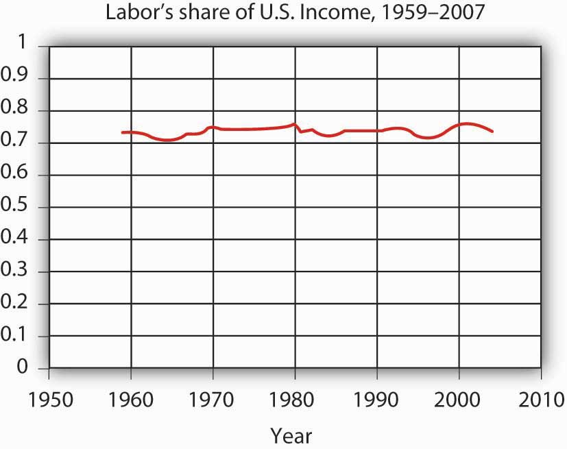
Labor generates considerably more income in the economy than all other factors of production combined. Figure 12.1 “Labor’s Share of U.S. Income, 1959–2007” shows the share of total income earned annually by workers in the United States since 1959. Labor accounts for roughly 73% of the income earned in the U.S. economy. The rest is generated by owners of capital and of natural resources.
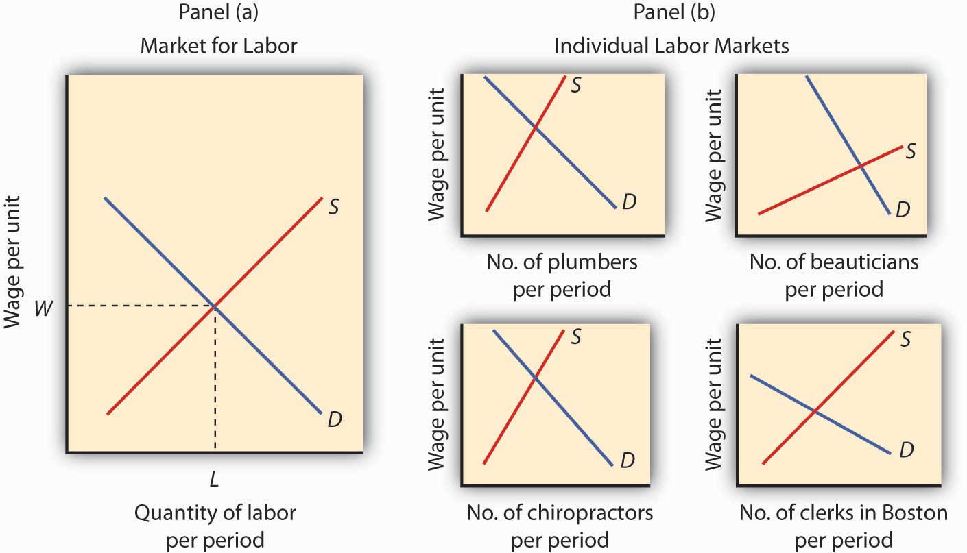
We calculate the total income earned by workers by multiplying their average wage times the number of workers employed. We can view the labor market as a single market, as suggested in Panel (a) of Figure 12.2 “Alternative Views of the Labor Market”. Here we assume that all workers are identical, that there is a single market for them, and that they all earn the same wage, W; the level of employment is L. Although the assumption of a single labor market flies wildly in the face of reality, economists often use it to highlight broad trends in the market. For example, if we want to show the impact of an increase in the demand for labor throughout the economy, we can show labor as a single market in which the increase in demand raises wages and employment.
Figure 12.2 Alternative Views of the Labor Market
One way to analyze the labor market is to assume that it is a single market with identical workers, as in Panel (a). Alternatively, we could examine specific pieces of the market, focusing on particular job categories or even on job categories in particular regions, as the graphs in Panel (b) suggest.
But we can also use demand and supply analysis to focus on the market for a particular group of workers. We might examine the market for plumbers, beauticians, or chiropractors. We might even want to focus on the market for, say, clerical workers in the Boston area. In such cases, we would examine the demand for and the supply of a particular segment of workers, as suggested by the graphs in Panel (b) of Figure 12.2 “Alternative Views of the Labor Market”.
Macroeconomic analysis typically makes use of the highly aggregated approach to labor-market analysis illustrated in Panel (a), where labor is viewed as a single market. Microeconomic analysis typically assesses particular markets for labor, as suggested in Panel (b).
When we use the model of demand and supply to analyze the determination of wages and employment, we are assuming that market forces, not individuals, determine wages in the economy. The model says that equilibrium wages are determined by the intersection of the demand and supply curves for labor in a particular market. Workers and firms in the market are thus price takers; they take the market-determined wage as given and respond to it. We are, in this instance, assuming that perfect competition prevails in the labor market. Just as there are some situations in the analysis of markets for goods and services for which such an assumption is inappropriate, so there are some cases in which the assumption is inappropriate for labor markets. We examine such cases in a later chapter. In this chapter, however, we will find that the assumption of perfect competition can give us important insights into the forces that determine wages and employment levels for workers.
We will begin our analysis of labor markets in the next section by looking at the forces that influence the demand for labor. In the following section we will turn to supply. In the final section, we will use what we have learned to look at labor markets at work.


